A Gentle & Intuitive Introduction to Linear Equations

Yashmeet Singh · Aug 5, 2024 · 8 minute read

Introduction

If you ask me, ”Where do I begin in my quest to become a data scientist?” I’ll say, ”linear equations”, without batting an eye.

It’s a simple technique that anyone who knows basic algebra and geometry can understand. But it teaches a crucial lesson in data analysis — how to interpret and visualize relationship between variables. And a solid grasp of linear equations sets the stage for linear regression, the first Machine Learning (ML) algorithm most people encounter.

In this article, I’ll explain linear equations step by step using examples. By the end, you’ll have an intuitive understanding of this fundamental concept, and feel confident to use it for more challenging problems.

Linear Relationship

Imagine you are at your favorite amusement park, where each ride costs $5. You’ll pay $10 for 2, $15 for 3 rides, and so on. In other words, the total cost varies proportionally with the number of rides. The below table shows the cost of up to 6 rides:

We can visualize this information by plotting the number of rides on the x-axis and the corresponding total cost on the y-axis:

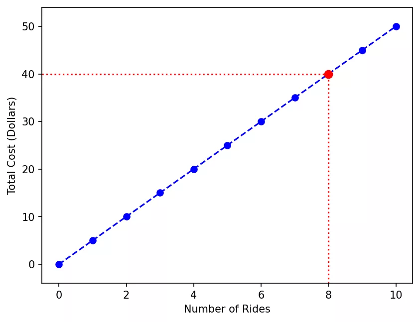
The graph shows a straight line (dashed blue), indicating that the two variables (ride count & total cost) are linearly related or have a linear relationship.

The line serves another crucial purpose. It can be used to calculate the total cost of an unknown number of rides.

Recall that the table had data only up to 6 rides. I’ve drawn the line using the table data and extended it to 10 on the x-axis. You can now use the line to find cost for upto 10 rides. For example, the below steps will get you the cost for 8 rides:

• Draw a vertical line from the x-axis at 8 rides.
• Locate the point where the vertical line meets the cost line (red dot).
• Plot a horizontal line from the red dot. The point where it meets the y-axis is the answer.
• Hence you’ll need to pay $40 for 8 rides.

This process of projecting known data to predict values in the unknown range is called extrapolation.

Linear Equation

We can also write the rides versus cost relationship as a simple equation:

$$Total \medspace Cost = 5 \times (Number \medspace of \medspace Rides)$$

The total cost depends on the number of rides, meaning the cost changes in response to ride count. Thus, the number of rides is the independent variable, and the total cost is the dependent variable.

The slope or coefficient is the rate at which the dependent variable changes with respect to a given independent variable. In our case, the cost goes up by $5 for each ride. Hence the variable number of rides has a slope of 5.

Let’s use the equation to find the cost of 8 rides:

It’s $40, which is the same result we got by extrapolating the line in the last section.

The Intercept

How about we add a little twist to our ride and cost relationship?

Suppose the amusement park has an admission fee of $20. Once you’ve paid this one-time fee to get in, each ride will still cost $5. We’ll need to update our linear equation to reflect this flat fee:

$$Total \medspace Cost = 20 + 5\times(Number \medspace of \medspace Rides)$$

Here’s the table with the updated cost for up to 6 rides:

Let’s plot this information as before - the number of rides goes on the x-axis and the total cost on the y-axis:

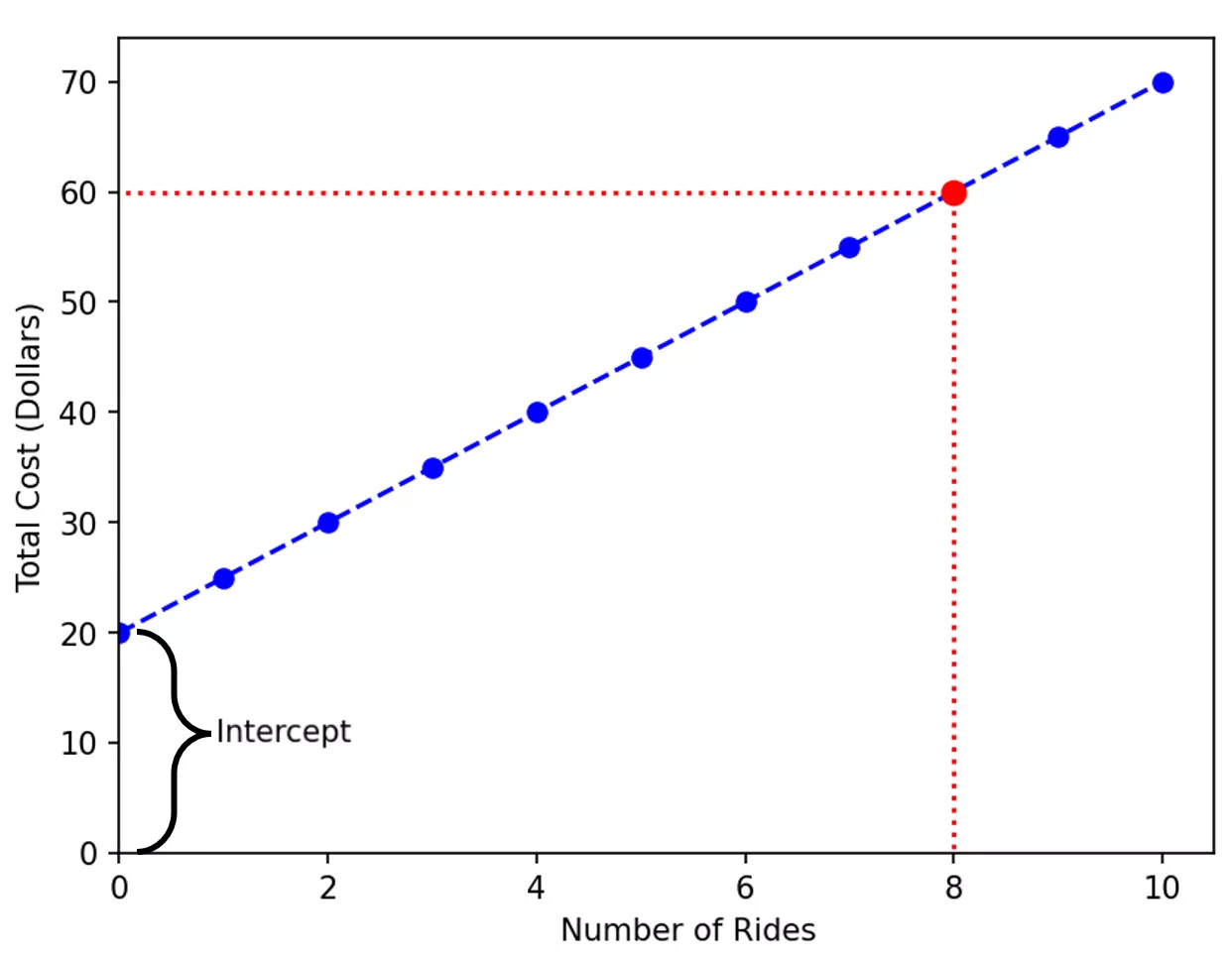
The ride-cost relationship is still a straight line (in dashed blue). But the line has been shifted up by a constant and now intersects the y-axis at 20. That’s the effect of the admission fee - you’ll pay $20 even if you don’t take any rides.

In general, the point where a linear equation meets the y-axis is known as y-intercept or just intercept. Therefore, the equation for the total cost has an intercept of 20.

Let’s calculate the revised cost for 8 rides. Again, you can use two methods. Either plug the number of rides in the new equation:

Or extrapolate using the updated graph as we did before. Both ways will lead you to the same result: $60.

The General Form

Let’s take another look at the equation from the last section:

Typically, the letters $\textbf{\textit{x}}$ and $\textbf{\textit{y}}$ are used to represent independent and dependent variables, respectively. Let’s rewrite our equation using this convention:

$$y = 20 + 5x$$

where $x$ = number of rides, $y$ = total cost.

The equation above contains two constants: the y-intercept (20) and the coefficient (5). These constants are usually denoted by the letters $\textbf{\textit{b}}$ and $\textbf{\textit{m}}$, respectively.

Let’s use these letters for the constants. Now our equation looks like below:

$$y = b + mx$$

We can rearrange the terms on the right side. That’ll give us the general form of the linear equation:

$$y = mx + b$$

Multiple Independent Variables

Suppose you see an ice cream truck at the park and decide to have a few cones of your favorite flavor between the rides. Each cone costs $3.

Now, the linear equation to calculate the total cost will have 3 variables - 2 independent (rides & ice cream cones) and 1 dependent (total cost). Here’s the updated equation:

When there are multiple independent variables, we typically use $x$ with subscripts ($x_{1}$, $x_{2}$, $x_{3}$ ..) to represent them. Thus, our equation can rewritten as:

$$y = 20 + 5x_1 + 3x_2$$

where:

• $x_1$ and $x_2$ are the independent variables for the counts of rides and ice cream cones, respectively.
• $y$ is the dependent variable, representing the total cost.
• The constant 20 is the intercept (i.e., the value of $y$ when both $x_1$ and $x_2$ are zero).
• The constants 5 and 3 are the coefficients or slopes for the variables $x_1$ and $x_2$, respectively. It means the total cost increases by 5 dollars for an additional ride, and by 3 dollars for each ice cream cone consumed.

Plotting Multiple Variables

How can you visualize our new linear equation with 3 variables? We’ll need 3-dimensional (3D) space where two dimensions will be used for independent variables ($x_1$ and $x_2$) and the third for the dependent variable ($y$):

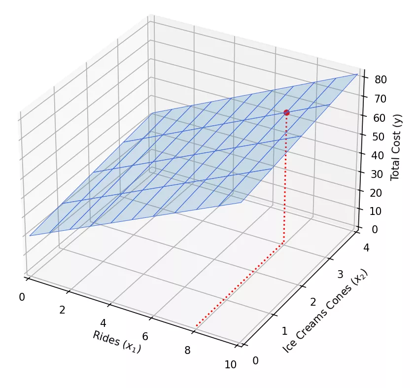
The total cost is now a flat surface or a plane (light blue shade). Each point on this plane represents the cost for a specific combination of rides ($x_1$) and ice cream cones ($x_2$)

Assignment: How much would it cost if you took 8 rides and had 3 ice cream cones? Find the answer using the equation. You can also visualize the answer using the 3D graph. Do both answers match?

What happens if a linear equation has 4 or more variables? Our brains are not equipped to visualize such higher dimensions. We’ll need to rely on our imagination instead.

We know that a linear equation with 2 variables is a line in a 2D space, and with 3 variables, it’s a plane in a 3D space. We can extend this idea - a linear equation with 4 or more variables can be thought of as a “hyperplane” in a high-dimensional space.

Negative Slope

So far, we’ve looked at variables that move in the same direction - if the number of rides increases, the total cost rises proportionally. The linear equations for such variables have a positive slope.

But what if the variables are inversely related? If one goes up, the other goes down accordingly. In this case, the slope will be negative, reflecting the reciprocal relationship between the variables.

Let’s take a example. Suppose you have $40 cash and pop into a grocery store to buy milk. One gallon of milk costs $4. If you buy one gallon, you’ll be left with $36; if you get 2 gallons, you’ll have $32, and so on.

The cash left is inversely proportional to the gallons of milk bought. Below equation captures this negative relationship:

$$y = 40 - 4x$$

where $x$ = gallons of milk purchased, $y$ = amount of cash left.

The slope is $-4$, indicating that $x$ and $y$ move in opposite directions: if $x$ increases, $y$ goes down proportionally.

Assignment:

• Draw the above linear equation in a 2D plot. How does a negative slope look in the graph?
• How much cash would be left if you bought 8 gallons of milk? Find the answer in two ways - using the equation and the graph. Do the answers match?

Summary

Wow, we covered a lot of ground in this article! Let’s recap what you learned today:

• What is a linear relationship?
• How do you write a linear relationship as an equation?
• What are indepedent and dependent variables?
• How to recognize and work with multiple indepedent variables in a linear relationship?
• How can you plot linear relationships in a 2D or 3D space?
• What is extrapolation, and why is it useful?
• What is the slope (or coefficient) of a linear equation? And what does it signify?

The above concepts are fundamental to data analysis and machine learning (ML). Now that you understand them intuitively, you are ready to dive into ML algorithms. Stay tuned for my upcoming article on linear regression which builds on this solid foundation and takes you further in your ML journey.

Happy learning!