· 7 minute read

3 Regression Metrics You Must Know: MAE, MSE, and RMSE
· · 9 minute read
Introduction
Let’s say you’ve built a new machine learning model. How do you know if it’s going to make good predictions?
How can you measure your model’s expected performance in the real world?
Today we’ll address this question for regression models. Specifically, we’ll look at three widely used regression metrics:
- Mean Absolute Error (MAE)
- Mean Squared Error (MSE)
- Root Mean Squared Error (RMSE)
Then I’ll show you how to calculate these metrics using Python and Scikit-Learn.
Let’s get started!
 Image Credit: Manfred Irmer
Regression Error
In statistics and machine learning, regression refers to a set of techniques used to predict a numerical value based on some inputs.
Suppose you want to train a model to predict airfare for US domestic flights. That would be a regression task because the output (airfare) can take on any value, say, from 1,000.
Once you’ve trained the model, you must measure its performance using a test dataset.
Let’s say we have a test dataset with 10 entries. We use the model to predict price for each entry. And then compare our predictions against the actual prices:
| Ticket # |
Actual Price |
Predicted Price |
|---|---|---|
| 1 | 250 | 265 |
| 2 | 110 | 140 |
| 3 | 500 | 480 |
| 4 | 200 | 215 |
| 5 | 330 | 290 |
| 6 | 490 | 515 |
| 7 | 670 | 750 |
| 8 | 210 | 210 |
| 9 | 435 | 420 |
| 10 | 375 | 285 |
How far off were our predictions from the actual prices? Let’s find out the prediction error for each entry using the below formula:
| Ticket # | Actual Price | Predicted Price | Error |
|---|---|---|---|
| 1 | 250 | 265 | -15 |
| 2 | 110 | 140 | -30 |
| 3 | 500 | 480 | 20 |
| 4 | 200 | 215 | -15 |
| 5 | 330 | 290 | 40 |
| 6 | 490 | 515 | -25 |
| 7 | 670 | 750 | -80 |
| 8 | 210 | 210 | 0 |
| 9 | 435 | 420 | 15 |
| 10 | 375 | 285 | 90 |
| Total | 0 |
The model over-predicted for some entries (in red). That is, the prediction was higher than the actual value. Thus the error is negative.
For other cases (in yellow), the model under-predicted as its prediction was lower than the actual value. Hence the error is positive.
Knowing individual errors for each entry is fine. But how can we combine all of these errors to give us one metric?
What if we add up all the errors? That won’t work. The negative errors would cancel out the positive errors.
For example, the sum of all errors in TABLE 2 is 0. That would lead us to believe that our model is perfect. That’s not true, though - the model made incorrect predictions for 9 out of 10 test cases!
Let’s try a different approach.
Mean Absolute Error (MAE)
As we saw above, the prediction error can be positive or negative. But what if we focus only on the size of the error and ignore the sign? That is, we measure the absolute value of the error.
In that case, we’ll treat two errors the same if they have equal size but only differ in sign (e.g., -80 and +80). Both are equally off from the expected value.
We can get absolute errors by dropping the sign from all the negative values:
| Ticket # | Actual Price | Predicted Price | Error | Absolute Error |
|---|---|---|---|---|
| 1 | 250 | 265 | -15 | 15 |
| 2 | 110 | 140 | -30 | 30 |
| 3 | 500 | 480 | 20 | 20 |
| 4 | 200 | 215 | -15 | 15 |
| 5 | 330 | 290 | 40 | 40 |
| 6 | 490 | 515 | -25 | 25 |
| 7 | 670 | 750 | -80 | 80 |
| 8 | 210 | 210 | 0 | 0 |
| 9 | 435 | 420 | 15 | 15 |
| 10 | 375 | 285 | 90 | 90 |
| Total | 0 | 330 |
And then divide the sum of absolute errors by the number of predictions. That’ll give us the Mean Absolute Error (MAE):
Let’s apply this formula to our example:
Thus, the MAE for our model is 33. The average difference between the predicted and actual ticket prices will be $33.
Mean Squared Error
MAE treats absolute errors linearly - a change in the error will have a proportional effect on MAE. For example, an error of 40 is twice as bad as an error of 20.
In reality, however, we want to build models that don’t generate larger errors too often. Thus we need a metric that penalizes larger errors more harshly than smaller ones.
Wc can create a metric using the square of errors. That’ll ensure that a larger error will produce a far more pronounced effect.
Consider two error values - 20 and 40. Their squared values are 400 and 1600, respectively. Even though 40 is twice of 20, it’ll contribute 4 times to the total squared error.
Let’s calculate the square of errors for the airfare model:
| Ticket # | Actual Price | Predicted Price | Error | Absolute Error | Squared Error |
|---|---|---|---|---|---|
| 1 | 250 | 265 | -15 | 15 | 225 |
| 2 | 110 | 140 | -30 | 30 | 900 |
| 3 | 500 | 480 | 20 | 20 | 400 |
| 4 | 200 | 215 | -15 | 15 | 225 |
| 5 | 330 | 290 | 40 | 40 | 1600 |
| 6 | 490 | 515 | -25 | 25 | 625 |
| 7 | 670 | 750 | -80 | 80 | 6400 |
| 8 | 210 | 210 | 0 | 0 | 0 |
| 9 | 435 | 420 | 15 | 15 | 225 |
| 10 | 375 | 285 | 90 | 90 | 8100 |
| Total | 0 | 330 | 18700 |
Dividing the sum of squared errors by the number of predictions will give us the Mean Squared Error (MSE):
Let’s apply this formula to our example problem:
Root Mean Squared Error (RMSE)
MSE is a helpful metric, but it is hard to interpret. It, by definition, involved squaring of error terms. Thus MSE doesn’t have the same units as the value we want to predict.
For example, the MSE for our airfare prediction model is 1870. We cannot report it in dollar terms: an MSE of 1870 is meaningless when the price range is 1,000.
It’s easy to convert MSE to a value that we can understand. Taking a square root of MSE will give us Root Mean Squared Error (RMSE):
Here’s the RMSE for our model:
This value makes sense. We can report that RMSE for our model is $43.24.
MAE vs. RMSE
Our model’s RMSE ($43.24) is significantly higher than the MAE ($33). Why is that?
Notice in TABLE 4 that we have two absolute errors (80 and 90) that are much larger than the others.
When we square all the errors to find RMSE, these two large errors dominate the others (see the last column in TABLE 4). Hence, they push RMSE to a considerably higher value than MAE.
This explains why RMSE would be a superior metric when we want to minimize larger errors.
Practice using Python & Scikit-Learn
Now you are familiar with the regression metrics MAE, MSE, and RMSE. Let’s learn how to calculate them using Python and Scikit-Learn.
Load Dataset
We’ll use a kaggle dataset that contains heights and weights measurements for 25,000 individuals.
We’ll first train a model to predict a person’s weight based on height. Then we’ll calculate the metrics to evaluate the model.
First off, let’s load the dataset using pandas:
import pandas as pd

dataset = pd.read_csv(
    'SOCR-HeightWeight.csv',
    # dataset has an extra index column. We don't need it.
    # Just load height and weight columns
    usecols=[1, 2]
)
dataset.info()
<class 'pandas.core.frame.DataFrame'>
RangeIndex: 25000 entries, 0 to 24999
Data columns (total 2 columns):
# Column Non-Null Count Dtype
--- ------ -------------- -----
0 Height(Inches) 25000 non-null float64
1 Weight(Pounds) 25000 non-null float64
dtypes: float64(2)
memory usage: 390.8 KBThe data types for both columns look good. And there are no missing values.
Next, use the seaborn scatterplot to see if heights and weights are associated:
import seaborn as sns

sns.scatterplot(
    x=dataset['Height(Inches)'],
    y=dataset['Weight(Pounds)'],
)
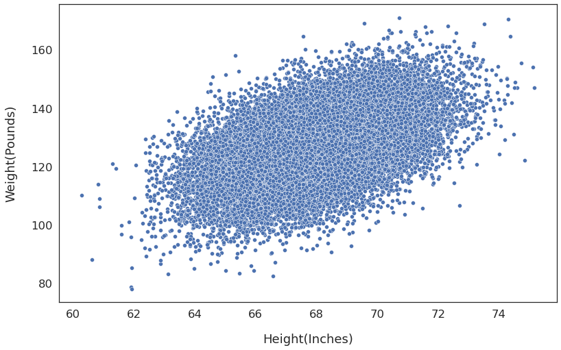
The weight generally goes up as the height increases. So a machine learning model should be able to capture this pattern and predict the weight with reasonable accuracy.
Build Regression Model
Let’s use linear regression to build the model. First, we store the inputs and output in separate variables:
# Input
X = dataset['Height(Inches)']
# Output
y = dataset['Weight(Pounds)']
Next, split the dataset into training and test sets. We’ll use the training set to build the model. And then evaluate the model using the test set.
from sklearn.model_selection import train_test_split

# 67% - training set (X_train, y_train)
# 33% - test set (X_test, y_test)
X_train, X_test, y_train, y_test = train_test_split(X, y, test_size=0.33)

# X_train and X_test are instances of pandas Series because
# they contain only one column. Convert them to DataFrames
X_train = X_train.to_frame()
X_test = X_test.to_frame()
Finally, create and train a model using Scikit-Learn’s LinearRegression:
from sklearn.linear_model import LinearRegression
# Create a new model
model = LinearRegression()
# build the model using the traing data
model.fit(X_train, y_train)
Calculate Metrics - MAE, MSE, and RMSE
We now have a fully trained model. Its time to measure it’s performance using the metrics we learned today.
First, let’s predict the weights for the test set:
predicted = model.predict(X_test)

actual_vs_predicted = pd.DataFrame(
    {'Actual': y_test,
     'Predicted':predicted}
)
# Show first 5 rows
actual_vs_predicted.head().round(2)| Actual | Predicted | |
|---|---|---|
| 7799 | 127.88 | 126.79 |
| 4427 | 108.97 | 117.22 |
| 14941 | 122.29 | 127.96 |
| 11644 | 118.53 | 124.57 |
| 15548 | 120.58 | 126.88 |
Scikit-Learn provides built-in functions to calculate a variety of metrics. Let’s import two of them we’ll use today:
from sklearn.metrics import (
    mean_absolute_error, # MAE
    mean_squared_error # MSE
)
First, we’ll compute Mean Absolute Error (MAE) using the function mean_absolute_error:
MAE = mean_absolute_error(
    y_true=y_test, # actual values
    y_pred=predicted # predicted values
)
MAE.round(2)8.06And then calculate Mean Squared Error (MSE) using mean_squared_error:
MSE = mean_squared_error(
    y_true=y_test, # actual values
    y_pred=predicted # predicted values
)
MSE.round(2)102.62Scikit-Learn doesn’t provide a function to provide Root Mean Squared Error (RMSE). But we can get RMSE by taking a square root of MSE:
# Square root of MSE gives RMSE
RMSE = MSE**(1/2)
RMSE.round(2)10.13Thus our model will predict weights with MAE and RMSE of 8.06 and 10.13 pounds, respectively.
Summary & Next Steps
This post introduced the most commonly used metrics to evaluate regression models. Let’s recap what you learned today:
- What is regression prediction error?
- How to use prediction errors to calculate MAE, MSE, and RMSE.
- MAE vs. RMSE: what’s the difference, and why does it matter?
- How to compute these metrics using Python and Scikit-Learn’s built-in functions.
Now that you know regression metrics, you might wonder: what about classification models - how do I evaluate them? You can learn all about that here and here.
Title Image by
babilkulesi