· 6 minute read

Use Standard and MinMax Scaling to Tame Numerical Features
· · 6 minute read
Features with vastly different scales can lead to subpar models. Here's how Standard and MinMax scalers can help.
Introduction
Imagine you’re in a bar catching up with a long-lost friend. You would love to know what he’s been up to lately.
There’s only one problem, though. The music is too loud to talk. It completely drowns out your friend’s voice. Your brain struggles to process any sound of much lower volume than the booming music.

Your machine learning model could run into a similar problem if it encounters features with significantly different scales1. It may not pick enough signal from features with a smaller scale.
To avoid this, we need to scale features. That is, we must transform them so that they have similar scales.
Let’s explore two popular scaling methods - Standard and MinMax scaling.
The Dataset
We’ll work with the real estate valuation dataset and focus on three numerical features:
age: the age of the house in yearsstation_distance: distance to the closest train stationstores_count: the number of convenience stores within walking distance
import pandas as pd

full_df = pd.read_csv("taiwan_real_estate.csv")

# work with a sample of 100 rows to keep the plots clutter free
real_estate_df = full_df.sample(100, ignore_index=True)
real_estate_df = real_estate_df[['age', 'station_distance', 'stores_count']]
real_estate_df.head()| age | station_distance | stores_count | |
|---|---|---|---|
| 0 | 32.1 | 1438.5790 | 3 |
| 1 | 34.9 | 567.0349 | 4 |
| 2 | 33.0 | 181.0766 | 9 |
| 3 | 13.6 | 4197.3490 | 0 |
| 4 | 32.0 | 1156.7770 | 0 |
Why Should You Scale Features?
Let’s look at a few statistics for our features:
| Min | Max | Range | Mean | Standard Deviation |
|
|---|---|---|---|---|---|
| age | 0.00 | 43.80 | 43.80 | 19.36 | 11.87 |
| station_distance | 49.66 | 6396.28 | 6346.62 | 1084.08 | 1365.53 |
| stores_count | 0.00 | 10.00 | 10.00 | 4.16 | 2.80 |
The feature station_distance has a much larger scale than the other features. Its range, mean and standard deviation are about 100 times greater than the others.
The plot below makes this point very clear:
import matplotlib.pyplot as plt
import seaborn as sns

sns.lineplot(data=real_estate_df)
plt.title('Raw Features: Line Plot')
plt.xlabel("Index")
plt.ylabel("Values")
plt.show()
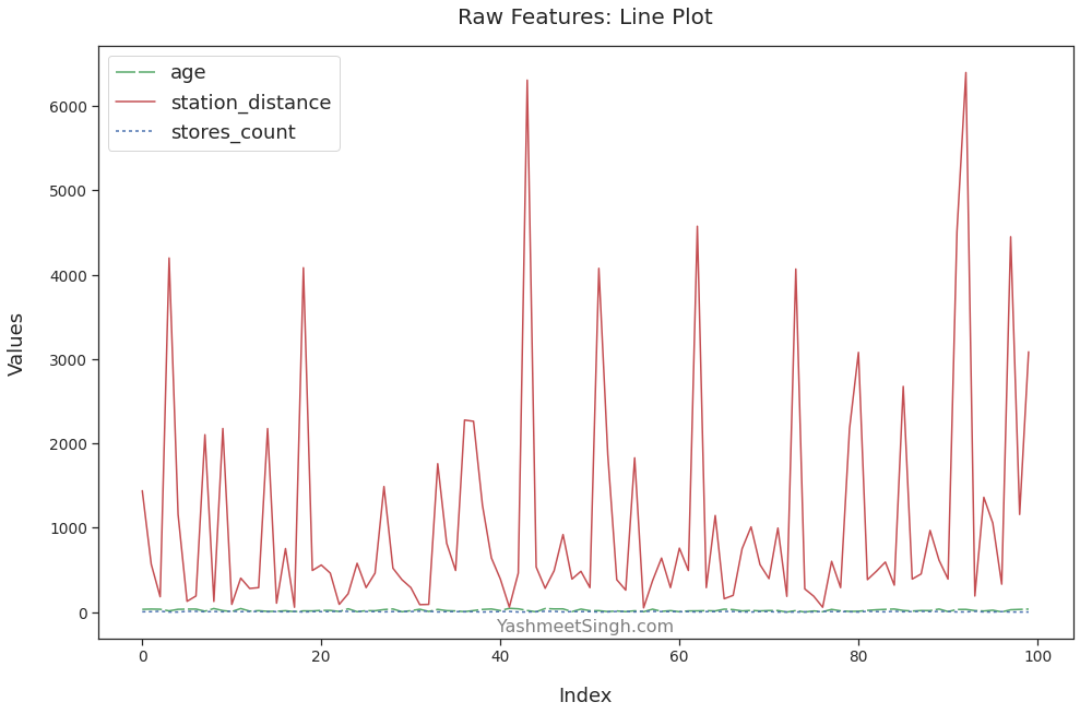
We can see all the variations in the value of station_distance. It mostly stays under 1000. But there are spikes when its value is much higher, going all the way to over 6000.
We don’t see such details for other features. The plots for age and stores_count are almost straight lines with barely any variations. That’s because they have much smaller scales than station_distance.
Essentially, the louder feature station_distance has muted age and stores_count. That will cause problems when we train a model on this data.
Most machine learning algorithms find the optimal solution by iteratively trying different values of parameters. This process is called Gradient Descent.
If you have a feature with a bigger scale, Gradient Descent will take larger steps to find the best possible parameter values. Therefore, our model will fail to learn from the nuances and variations of features with a much smaller scale.
We can fix this issue by scaling features before we train the model.
Standard Scaling
Standard scaling transforms features so that their mean becomes 0 and their standard deviation is 1.
It does so by asking a simple question. How far is each data point from the mean? More precisely, it measures this distance in terms of the standard deviation using the below formula:
For example, let’s calculate the scaled value for the first data point of the feature station_distance:
- Feature’s mean is 1084.08, and the standard deviation is 1365.53
- The first data point is 1438.579
- The scaled value is
We’ll need to repeat this for each data point of every feature.
Sklearn’s StandardScaler can do all of that in a few lines of code:
from sklearn.preprocessing import StandardScaler

standard_scaler = StandardScaler()

# calculate mean and standard deviation for each feature
standard_scaler.fit(real_estate_df)

# scale each feature using its mean and standard deviation
scaled_df = standard_scaler.transform(real_estate_df)

# convert to dataframe for illustrative purposes
scaled_df = pd.DataFrame(scaled_df, columns=real_estate_df.columns)
Let’s print statistics for the scaled features:
| Min | Max | Range | Mean | Standard Deviation |
|
|---|---|---|---|---|---|
| age | -1.64 | 2.07 | 3.71 | 0.00 | 1.01 |
| station_distance | -0.76 | 3.91 | 4.67 | -0.00 | 1.01 |
| stores_count | -1.49 | 2.09 | 3.59 | -0.00 | 1.01 |
As expected, the scaled features have their mean set to 0 and standard deviation to 1.
Here’s the line plot for the scaled features:
sns.lineplot(data=scaled_df)

plt.title('Standard Scaling: Line Plot')
plt.xlabel("Index")
plt.ylabel("Values")
plt.show()
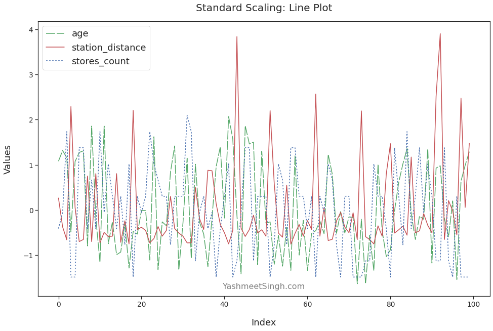
We can see age and stores_count in greater detail. The variations in their values - peaks and valleys - are plain to see now. Moreover, all the features have comparable ranges.
Our model can now learn from all the features to find the best fitting solution.
Let’s look at one more way to scale the features.
MinMax Scaling
Standard scaling works by making mean and standard deviation the same for all the features.
MinMax scaling focuses on the range instead. It ensures that all the features will have the same range of 0 to 1. It does so using the below formula:
Let’s perform MinMax scaling for the first data point of the feature station_distance:
- Feature’s minimum is 49.66 and maximum is 6396.283
- The first data point is 1438.579
- The scaled value is
We’ll use sklearn’s MinMaxScaler to do this for all features:
from sklearn.preprocessing import MinMaxScaler

minmax_scaler = MinMaxScaler()

# calculate minimum and maximum for each feature
minmax_scaler.fit(real_estate_df)

# scale each feature using its minimum and maximum values
minmax_scaled_df = minmax_scaler.transform(real_estate_df)

# convert to dataframe for illustrative purposes
minmax_scaled_df = pd.DataFrame(minmax_scaled_df,
                                columns=real_estate_df.columns)
Let’s print statistics for the scaled features:
| Min | Max | Range | Mean | Standard Deviation |
|
|---|---|---|---|---|---|
| age | 0.00 | 1.00 | 1.00 | 0.44 | 0.27 |
| station_distance | 0.00 | 1.00 | 1.00 | 0.16 | 0.22 |
| stores_count | 0.00 | 1.00 | 1.00 | 0.42 | 0.28 |
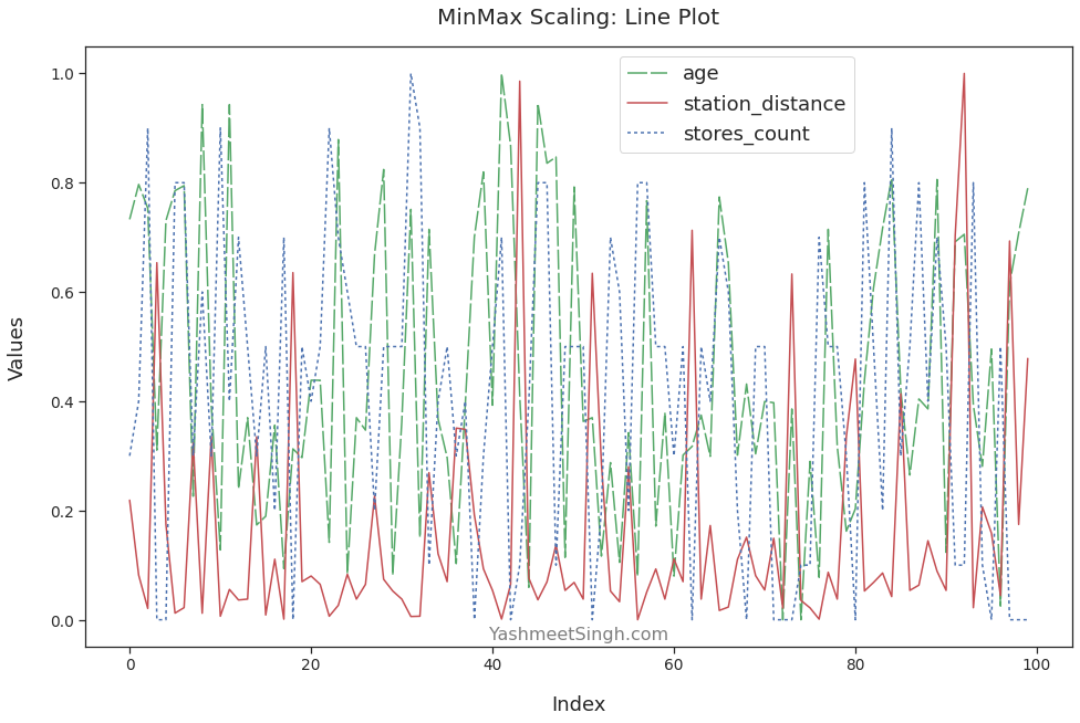
As expected, all the scaled features have the same range. Their minimum and maximum values are 0 and 1, respectively.
The line plot confirms this as well:
ax = sns.lineplot(data=minmax_scaled_df)

plt.title('MinMax Scaling: Line Plot')
plt.xlabel("Index")
plt.ylabel("Values")
# use bbox_to_anchor to move legend
# so that it doesn't cover line plots
plt.legend(loc='upper center', bbox_to_anchor=(0.65, 1))
plt.show()
Conclusion
It’s usually a bad idea to train models on features with vastly different scales.
We should scale such features before training a model. We explored two ways to do that.
Standard scaling moves every feature’s mean to 0 and standard deviation to 1. The scaled features will also have comparable ranges.
MinMax scaling transforms all the features to have the same range (from 0 to 1).
Final Thought
Standard and MinMax scalers are great tools to handle numerical features. But they have a limitation.
They don’t do well with features containing outliers. That’s because mean and range are highly sensitive to outliers. Even one extreme value can change a feature’s mean and range significantly.
So what’s our alternative?
We may want to scale features using statistics that are resistant to outliers. Check out the post where I discuss this in detail.
Footnotes
-
Think of scale as the range of the feature values. And how those values are distributed within that range. ↩
Title Image by
Pexels