· 6 minute read

Use ‘Train Test Split’ to Beat Overfitting
· · 10 minute read
Here's how you can stop overfitting dead in it's tracks and train your models with confidence.
Introduction
When you’re building a new machine learning model, you can fine-tune it to gain more insights from the training data.
The trick is to know when to stop fine-tuning.
After a certain point, the model will start to overfit. That is, it may perform well on the training data. But it’ll give disappointing results when it encounters unseen data.
How do you stop overfitting? How can you measure your model’s expected performance in the real world?
The ‘train test split’ technique is the answer to these questions. Let’s explore what it is and how to use it.
The Dataset
We’ll work on the Combined Cycle Power Plant Data Set. Here’s the official description:
“The dataset contains 9568 data points collected from a Combined Cycle Power Plant over 6 years (2006-2011), when the power plant was set to work with full load.
Features consist of hourly average ambient variables Temperature (T), Ambient Pressure (AP), Relative Humidity (RH) and Exhaust Vacuum (V) to predict the net hourly electrical energy output (EP) of the plant.”
Imagine the power plant hired us to build a model to predict the energy output.
Let’s start by loading the dataset:
import pandas as pd

dataset = pd.read_csv("power_plant.csv")
dataset.head()| temperature | exhaust_vacuum | pressure | humidity | output_mw | |
|---|---|---|---|---|---|
| 0 | 14.96 | 41.76 | 1024.07 | 73.17 | 463.26 |
| 1 | 25.18 | 62.96 | 1020.04 | 59.08 | 444.37 |
| 2 | 5.11 | 39.40 | 1012.16 | 92.14 | 488.56 |
| 3 | 20.86 | 57.32 | 1010.24 | 76.64 | 446.48 |
| 4 | 10.82 | 37.50 | 1009.23 | 96.62 | 473.90 |
dataset.info()<class 'pandas.core.frame.DataFrame'>
RangeIndex: 9568 entries, 0 to 9567
Data columns (total 5 columns):
# Column Non-Null Count Dtype
--- ------ -------------- -----
0 temperature 9568 non-null float64
1 exhaust_vacuum 9568 non-null float64
2 pressure 9568 non-null float64
3 humidity 9568 non-null float64
4 output_mw 9568 non-null float64
dtypes: float64(5)
memory usage: 373.9 KBThe dataset looks good. There are 9568 observations, and we don’t have any missing data.
We move on to model building.1
Using Entire Dataset for Training
You might be tempted to train a new model on the entire dataset. After all, the more data you use for training, the better your model will be. Right?
We’ll find out soon what’s wrong with that approach. But let’s give it a try anyway.
First, we separate features (input) from the labels (output):
X = dataset.drop(columns='output_mw') # features or input
y = dataset.loc[:, 'output_mw'] # label or output
Let’s assume you’ve decided to use Polynomial Regression. Your next task is to find the polynomial degree that’ll deliver the best predictions.
We’ll perform these steps to create and evaluate our model:
- Generate polynomial terms for the features
X. - Scale the polynomial terms.
- Train a linear regression model on the scaled terms.
- When the model is fully trained, use it to predict output for
X. - Compare predictions with the known labels
yto calculate Root Mean Squared Error (RMSE).
We’ll create multiple models - one for each polynomial degree 1 to 12. We’ll choose the model which minimizes RMSE.
from sklearn.linear_model import LinearRegression
from sklearn.metrics import mean_squared_error
from sklearn.pipeline import make_pipeline
from sklearn.preprocessing import PolynomialFeatures
from sklearn.preprocessing import StandardScaler

rmse_list = []

# runs from degree = 1 to 12
for degree in range(1, 13):

    # Use pipeline to perform these steps in sequence
    pipeline_steps = [
        PolynomialFeatures(degree=degree),
        StandardScaler(),
        LinearRegression()
    ]
    pipeline = make_pipeline(*pipeline_steps)

    # train the model using X and y
    pipeline.fit(X, y)

    # predict output for X
    y_predictions = pipeline.predict(X)

    # compare predictions with labels y to calculate RMSE
    rmse = mean_squared_error(y, y_predictions)**(1/2)
    rmse_list.append(rmse)

# convert error list to dataframe. its easier to work with.
error_df = pd.DataFrame(
    {'RMSE': rmse_list},
    index=range(1, 13)
)
error_df.index.name = 'Degree'
Here’s the error (RMSE) versus the degree of the polynomial model:
error_df.round(2).transpose()| Degree | 1 | 2 | 3 | 4 | 5 | 6 | 7 | 8 | 9 | 10 | 11 | 12 |
|---|---|---|---|---|---|---|---|---|---|---|---|---|
| RMSE | 4.56 | 4.25 | 4.15 | 4.08 | 3.97 | 3.9 | 3.81 | 3.74 | 3.69 | 3.66 | 3.58 | 3.44 |
You can plot it as well:
import matplotlib.pyplot as plt
import seaborn as sns

plt.style.use('ggplot')

sns.lineplot(data=error_df, markers=True)
plt.title('Polynomial Model: Degree vs Error')
plt.xlabel("Degree")
plt.ylabel("Root Mean Squared Error (RMSE)")
plt.show()
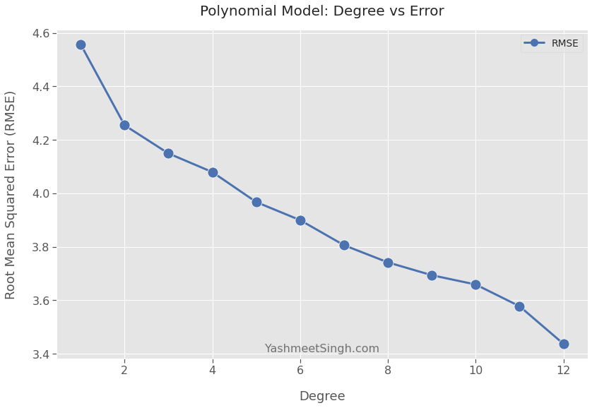
The trend is clear. The error goes down as the polynomial degree goes up.
The model built using degree 12 has the lowest error.2 Does that mean you should choose it as your final model?
Doing so will be a disaster, as we’ll find in the next section.
Using Train Test Split
So far, we have trained a model on the entire dataset. Then we measured the model’s performance using the same dataset.
In other words, we trained and tested the model on the same data.
Ideally, we want a model that learns general patterns from the training data and minimizes prediction error for unseen data.
The ‘train test split’ technique can help us with that. It splits the input dataset into two sets:
- Training set: Use it to train the model.
- Test set: This acts as the unseen data. Use it to evaluate the trained model.
Let’s see it in action.
The Split
We’ll use sklearn’s train_test_split. It’ll shuffle and then split the dataset into training and test sets.
We’ll set aside 25% of the observations for testing. We will use the rest for training the model.3
from sklearn.model_selection import train_test_split

X_train, X_test, y_train, y_test = train_test_split(X, y, test_size=0.25)
X_train and y_train form the training set. X_test and y_test are the test set.
Measuring Test Errors
Next, we’ll again build models of polynomial degrees 1 to 12.
We’ll add one more step to the list from the previous section.
After we train a model, we’ll use it to predict output for X_test.
We’ll compare these predictions with labels y_test to calculate test RMSE.
Since we won’t train models on X_test and y_test, test RMSE will reflect how models will behave in the real world.
Let’s run the loop:4
def build_polynomial_models(X_train, y_train, X_test, y_test, max_degree):

    train_RMSE_list = []
    test_RMSE_list = []

    # runs from degree = 1 to max_degree
    for degree in range(1, max_degree+1):

        pipeline_steps = [
            PolynomialFeatures(degree=degree),
            StandardScaler(),
            LinearRegression()
        ]
        pipeline = make_pipeline(*pipeline_steps)

        # train the model using X_train and y_train
        pipeline.fit(X_train, y_train)

        # Predict output for X_train
        train_predictions = pipeline.predict(X_train)
        train_RMSE = mean_squared_error(y_train, train_predictions)**0.5
        train_RMSE_list.append(train_RMSE)

        # Predict output for X_test (unseen data)
        test_predictions = pipeline.predict(X_test)
        test_RMSE = mean_squared_error(y_test, test_predictions)**0.5
        test_RMSE_list.append(test_RMSE)

    error_df = pd.DataFrame(
        {'Training RMSE': train_RMSE_list, 'Test RMSE': test_RMSE_list},
        index=range(1, max_degree+1)
    )
    error_df.index.name = 'Degree'

    return error_df
error_df = build_polynomial_models(X_train,y_train,X_test,y_test,12)Let’s print the training and test RMSE for each degree:
error_df.round(2)| Degree | Training RMSE | Test RMSE |
|---|---|---|
| 1 | 4.57 | 4.53 |
| 2 | 4.25 | 4.27 |
| 3 | 4.15 | 4.16 |
| 4 | 4.07 | 4.12 |
| 5 | 3.96 | 4.03 |
| 6 | 3.89 | 4.00 |
| 7 | 3.83 | 4.10 |
| 8 | 3.73 | 4.14 |
| 9 | 3.59 | 5.01 |
| 10 | 3.50 | 11.11 |
| 11 | 3.42 | 49.95 |
| 12 | 3.34 | 240.88 |
The model with degree 12 doesn’t look so good now.
Its test RMSE is over 72 times worse than its training RMSE. To say that it would fail in production would be a gross understatement!
Let’s find out what went wrong.
Overfit
As exptected, the training RMSE decreases as the polynomial degree increases.
The test RMSE, however, starts to creep up after degree 6. It increases slowly from degrees 7 to 9 (in yellow) and then explodes from degrees 10 to 12 (in red).
That’s because the model is overfitting from degrees 7 to 12. It has adapted well to the training data. It’s not learning much about the general problem we’re trying to solve.
As an analogy, imagine we signed up for a Biology 101 course. The instructor shared a problem set with us. This set has all the questions (and their answers) that’ll appear in the final exam.
Some students may focus on the problem set. They’ll try to memorize the answer to every question. They may not learn much about Biology but will most likely score high on the exam.
Our model has behaved the same way by essentially memorizing the training data.
In general, the model is overfitting when the test error goes up while the training error is trending down. See the plot below.
# Plot up to degree 9. Including higher degrees will expand the
# y scale dramatically, visually squeezing RMSE for lower degrees
sns.lineplot(data=error_df.loc[:9], markers=['o', 's'])

plt.title('Polynomial Model: Degree vs Error')
plt.xlabel("Degree")
plt.ylabel("Root Mean Squared Error (RMSE)")
plt.show()
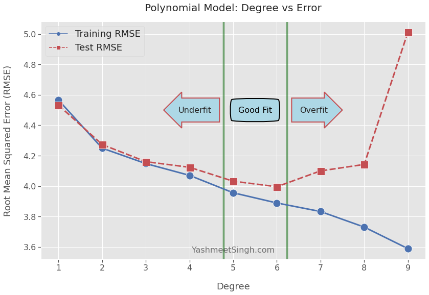
Underfit
Both training and test RMSE decrease for models with polynomial degrees 1 to 4.
The model is underfitting5 during this phase. The model hasn’t yet picked up enough signal from the training data.
We can continue training with higher degrees. We should stop when the test error either flatlines or begins to go up.
Good Fit
Now we only have models of degrees 5 and 6 to consider. We’re in a sweet spot where models have learned as much as they could from the training data.
The test RMSE scores for degrees 5 and 6 don’t differ by much. Moreover, moving to a degree lower or higher causes test RMSE to shoot up.
Now the question is - should we use degree 5 or 6 for our final model?
So far, we’ve been judging a model by its prediction error. We should consider one more thing: Can we explain predictions made by a model?
For example, our model may predict lower energy output. However, what if we want to know why the model predicted lower output?
Polynomial models become increasingly complex as the degree goes up. And complex models are harder to understand and explain.
If the reason for a prediction is important to you, you are better off choosing a simpler model. That’s especially true when the simpler model performs almost as well as the more complex model.
So, in our case, I would choose the model of polynomial degree 5.
Conclusion
We explored why we should always use train test split to train machine learning models.
We saw what happens when we use the entire dataset to train and test the model. Since we couldn’t evaluate the model on unseen data, the model overfitted to the dataset. Such a model will have serious performance issues when it encounters new inputs.
Then we built the model using the train test split technique. We set aside a portion of the dataset to evaluate the model. That helped us to detect and stop overfitting. So our final model will hold up well in the real world.
Footnotes
-
I’ve skipped exploratory data analysis because that’s not the focus of this post. Please don’t skip it for a real project! ↩
-
You can go with higher degrees, and you’ll notice the same trend. The RMSE for the training data will keep going down. ↩
-
The test set is typically 20% to 40% of the entire dataset. ↩
-
For convenience, I’ve created a method to run the loop from degrees 1 to 12. You can use it for any other dataset. ↩
-
Underfitting is not as serious an issue as overfitting. Here’s why:
When a model underfits, both training and test errors move in the same direction (both decrease). Moreover, they may not differ by much. So if an underfitting model performs poorly for unseen data, it doesn’t surprise you.
But when a model overfits, training and test errors move in opposite directions and may have a big gap. Therefore an overfitted model can blindside you with subpar results in production. ↩
Title Image by
denfran