· 8 minute read
Measures of Spread: MAD, Variance, and Standard Deviation
· · 7 minute read
Introduction
We recently learned how to find the central or the typical value of a given data set. This post focuses on metrics to measure how the data is spread around the center.
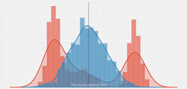
Let’s look at a motivating example. Consider that we have two datasets with the same mean (50). That doesn’t tell us how values are distributed in each dataset.
We could get a clue by drawing their histograms:
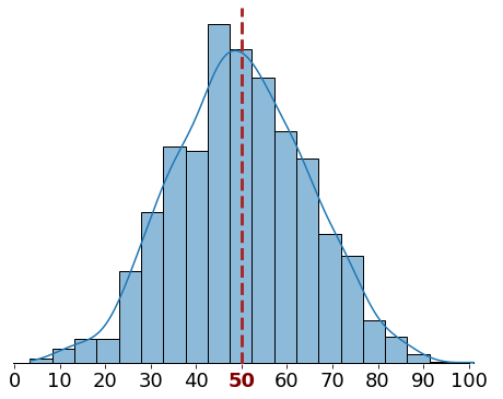
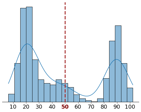
In the first dataset, most of the values are bunched tightly around the mean. In contrast, the second dataset has two clusters far from the mean.
The average distance from the mean will be much higher for the second dataset. That’s true even though both datasets have the same mean!
Now you might be asking - “how do I quantify this average, or typical, distance from the mean?”
This post will teach you three metrics to measure this distance:
- Variance
- Standard Deviation
- Mean Absolute Deviation (MAD)
Let’s get started!
Deviations from the Mean
Before calculating the metrics mentioned above, we need to find the distance, or deviation, of each score from the mean.
Allow me to illustrate this using an example.
Imagine you’re a science teacher at a high school. Here are the exams scores for the ten students in your class:
Let’s first calculate the mean score:
Next, we want to find out the deviation of each score using the below formula:
| Student # | Score | Deviation |
|---|---|---|
| 1 | 56 | -24 |
| 2 | 99 | 19 |
| 3 | 97 | 17 |
| 4 | 100 | 20 |
| 5 | 59 | -21 |
| 6 | 62 | -18 |
| 7 | 97 | 17 |
| 8 | 70 | -10 |
| 9 | 60 | -20 |
| 10 | 100 | 20 |
The scores below the mean generate negative deviations (in reddish shades). Similarly, positive deviations (in greenish shades) represent the scores above the mean.
How do we aggregate these deviations to get a single value to convey the average spread of the data?
We could find the mean of the deviations. Let’s try that:
What happened here? We know that none of the deviations were equal to zero. So why is the sum of deviations zero?
The mean, by definition, represents the middle balancing point of a dataset. The negative and positive deviations from the mean will cancel each other out. The deviations from the mean will always add up to zero.
Therefore, we cannot measure the average spread of a dataset by simply adding the deviations.
Let’s try a different approach.
Variance
We know that squaring a negative will always give us a positive result. Let’s square the deviations from the mean we calculated in the last section.
All the resulting squared deviations are positive (The last column below is all green). Therefore they won’t cancel each other out when we add them up:
| Student # | Score | Deviation | Squared Deviation |
|---|---|---|---|
| 1 | 56 | -24 | 576 |
| 2 | 99 | 19 | 361 |
| 3 | 97 | 17 | 289 |
| 4 | 100 | 20 | 400 |
| 5 | 59 | -21 | 441 |
| 6 | 62 | -18 | 324 |
| 7 | 97 | 17 | 289 |
| 8 | 70 | -10 | 100 |
| 9 | 60 | -20 | 400 |
| 10 | 100 | 20 | 400 |
| Total | 0 | 3580 |
Next, we can take the mean of the squared deviations. That’ll give us the variance.
Let’s calculate it for the student’s scores:
So the variance of the student’s score is 358.
Standard Deviation
Variance is a popular metric to measure spread, but it is hard to interpret. It involves squaring of deviations and thus doesn’t have the same units as the input values.
For example, the variance of student scores is 358. We cannot compare it to the scores’ mean (80) or range (56-100).
Luckily, that’s an easy problem to solve. We can take the square root of the variance to get the Standard Deviation:
Let’s calculate it for the student scores:
This value makes sense. The Standard Deviation of 18.92 represents how far a typical score is from the mean value (80).
Median Absolute Deviation (MAD)
Recall that the sum of raw deviations from the mean will always be zero. We squared the deviations to get around that problem.
There’s another way to ensure deviations don’t cancel each other out.
We can take the absolute values of the deviations. That means we’ll focus only on the size of the deviations and drop the sign from all the negative values.
Let’s apply this method to the student’s scores. The last column in the below table shows the absolute deviations:
| Student # |
Score | Deviation | Squared Deviation |
Absolute Deviation |
|---|---|---|---|---|
| 1 | 56 | -24 | 576 | 24 |
| 2 | 99 | 19 | 361 | 19 |
| 3 | 97 | 17 | 289 | 17 |
| 4 | 100 | 20 | 400 | 20 |
| 5 | 59 | -21 | 441 | 21 |
| 6 | 62 | -18 | 324 | 18 |
| 7 | 97 | 17 | 289 | 17 |
| 8 | 70 | -10 | 100 | 10 |
| 9 | 60 | -20 | 400 | 20 |
| 10 | 100 | 20 | 400 | 20 |
| Total | 0 | 3580 | 186 |
Next, divide the sum of these absolute values by the number of scores. That’ll give us the Mean Absolute Deviation (MAD):
Thus, the Mean Absolute Deviation for the students’ scores is 18.6 points.
Summary & Next Steps
Today you learned how to calculate Mean Absolute Deviation (MAD), Variance, and Standard Deviation for any given data set.
These metrics are known as the Measures of Spread because they represent the distance between a typical value and the center of the data.
Here’s how you can build upon the knowledge you gained today:
- Measures of spread play a crucial role in preparing numerical data for machine learning projects. You can read all about it here and here.
- Learn how to visualize data distributions using histograms and density curves.