· 15 minute read

Pandas 101: A Practical Guide for Absolute Beginners
· · 15 minute read
In a hurry to learn Pandas? Here's all you need to know to get started!
Introduction
Pandas is the most popular Python library for data analysis. It can easily handle large, messy datasets you’ll find in the real world. You can use its numerous functions to load and manipulate data and even create graphical plots.
Today, I’ll introduce Pandas basics and its most frequently used features. You’ll learn how to:
- Load tabular data (e.g., CSV file).
- Get summary statistics for numerical and categorical data.
- Manipulate columns - rename, remove, or add new columns.
- Sort and filter data.
- Group data and calculate aggregated results.
- Visualize data using Pandas (ex. bar, pie charts).
The Retail Sales Dataset
Before we start, let’s look at the dataset we’ll use in this article.
The retail sales dataset contains a fictitious store’s sales and profits for two consecutive quarters (Q3 and Q4). It breaks down this data by store departments and categories.
Here’s a screenshot of the entire dataset:
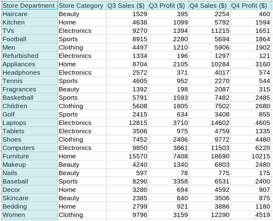
The first row contains the column labels. The store departments listed in the first column are unique. So we would like to use them as the index.
The data is stored in a CSV file named retail_sales_profits.csv. Let’s load and analyze it using Pandas.
Load the Dataset
First, we need to import Pandas. We usually do that using the alias pd:
import pandas as pdYou can use Pandas to load data from a variety of sources (ex., CSV, Excel, SQL database, HTML table, etc.)1.
Since our dataset is a CSV file, we’ll use the method read_csv(). It’ll return a DataFrame object. DataFrame is a 2-dimensional array Pandas uses to store tabular data.
# Read the CSV file into the 'sales_df' object (Sales DataFrame)
sales_df = pd.read_csv('retail_sales_profits.csv')
Let’s print the DataFrame object:2
sales_df| Store Department | Store Category | Q3 Sales ($) | Q3 Profit ($) | Q4 Sales ($) | Q4 Profit ($) | |
|---|---|---|---|---|---|---|
| 0 | Haircare | Beauty | 1529 | 395 | 2254 | 460 |
| 1 | Kitchen | Home | 4638 | 1099 | 5792 | 1594 |
| 2 | TVs | Electronics | 9270 | 1394 | 11215 | 1651 |
| 3 | Football | Sports | 8915 | 2280 | 5694 | 1864 |
| 4 | Men | Clothing | 4497 | 1210 | 5906 | 1902 |
| ... | ... | ... | ... | ... | ... | ... |
| 20 | Baseball | Sports | 8290 | 3358 | 6531 | 2400 |
| 21 | Decor | Home | 3280 | 694 | 4592 | 907 |
| 22 | Skincare | Beauty | 2385 | 640 | 3506 | 875 |
| 23 | Bedding | Home | 2799 | 921 | 3886 | 1180 |
| 24 | Women | Clothing | 9796 | 3159 | 12290 | 4519 |
25 rows × 6 columns
Pandas used the first row from the CSV file for column labels (in blue). However, it automatically added an index (in red). Let’s print it:
# Print the DataFrame index
sales_df.index
RangeIndex(start=0, stop=25, step=1)It’s a numerical index ranging from 0 to 24. It’s not going to be helpful in our analysis. Instead, we want to set the first column, Store Department, as the index.
Let’s look at two ways to do that.
Set Index While Loading Data
You can use read_csv()’s parameter index_col to set a column as index:
sales_df = pd.read_csv(
    'retail_sales_profits.csv', # file to load dataset
    index_col='Store Department' # column to set as the index
)
sales_df| Store Category | Q3 Sales ($) | Q3 Profit ($) | Q4 Sales ($) | Q4 Profit ($) | |
|---|---|---|---|---|---|
| Store Department | |||||
| Haircare | Beauty | 1529 | 395 | 2254 | 460 |
| Kitchen | Home | 4638 | 1099 | 5792 | 1594 |
| TVs | Electronics | 9270 | 1394 | 11215 | 1651 |
| Football | Sports | 8915 | 2280 | 5694 | 1864 |
| Men | Clothing | 4497 | 1210 | 5906 | 1902 |
| ... | ... | ... | ... | ... | ... |
| Baseball | Sports | 8290 | 3358 | 6531 | 2400 |
| Decor | Home | 3280 | 694 | 4592 | 907 |
| Skincare | Beauty | 2385 | 640 | 3506 | 875 |
| Bedding | Home | 2799 | 921 | 3886 | 1180 |
| Women | Clothing | 9796 | 3159 | 12290 | 4519 |
25 rows × 5 columns
Change Index After Data is Loaded
You can also change the index after you’ve already read the dataset.
The below code reloads the CSV file. That’ll create the integer column that we don’t want:
sales_df = pd.read_csv('retail_sales_profits.csv')
# print the index
sales_df.index
RangeIndex(start=0, stop=25, step=1)We can use the DataFrame method set_index() to change the index to the correct column:
sales_df = sales_df.set_index('Store Department')
# print the index again
sales_df.index
Index(['Haircare', 'Kitchen', 'TVs', 'Football', 'Men', 'Refurbished',
'Appliances', 'Headphones', 'Tennis', 'Fragrances', 'Basketball',
'Children', 'Golf', 'Laptops', 'Tablets', 'Shoes', 'Computers',
'Furniture', 'Makeup', 'Nails', 'Baseball', 'Decor', 'Skincare',
'Bedding', 'Women'],
dtype='object', name='Store Department')The column Store Department is now set as the index.
Access Rows By Index
The regular Python and NumPy arrays provide you with only a numerical index. Pandas goes one step further. As we saw in the last section, it allows you to set columns with string data as the index.
You can use these string index labels to query the DataFrame using loc[].
For example, the below code snippets use loc[] to access specific Store Departments:
# Access a row (department) using the string index label
sales_df.loc['Haircare']
Store Category Beauty
Q3 Sales ($) 1529
Q3 Profit ($) 395
Q4 Sales ($) 2254
Q4 Profit ($) 460
Name: Haircare, dtype: object# Access rows for multiple departments
# Notice the use of double square brackets
sales_df.loc[['Tennis', 'Laptops']]| Store Category | Q3 Sales ($) | Q3 Profit ($) | Q4 Sales ($) | Q4 Profit ($) | |
|---|---|---|---|---|---|
| Store Department | |||||
| Tennis | Sports | 4605 | 952 | 2270 | 544 |
| Laptops | Electronics | 12815 | 3710 | 14602 | 4605 |
Head and Tail
If you want to take a quick peek at the DataFrame, you can use the methods head() and tail(). They’ll print the first and last five DataFrame rows, respectively:
# print first 5 rows
sales_df.head()| Category | Q3_Sales | Q3 Profit ($) | Q4 Sales ($) | Q4 Profit ($) | |
|---|---|---|---|---|---|
| Store Department | |||||
| Haircare | Beauty | 1529 | 395 | 2254 | 460 |
| Kitchen | Home | 4638 | 1099 | 5792 | 1594 |
| TVs | Electronics | 9270 | 1394 | 11215 | 1651 |
| Football | Sports | 8915 | 2280 | 5694 | 1864 |
| Men | Clothing | 4497 | 1210 | 5906 | 1902 |
# print last 5 rows
sales_df.tail()| Category | Q3_Sales | Q3_Profit | Q4_Sales | Q4_Profit | |
|---|---|---|---|---|---|
| Store Department | |||||
| Baseball | Sports | 8290 | 3358 | 6531 | 2400 |
| Decor | Home | 3280 | 694 | 4592 | 907 |
| Skincare | Beauty | 2385 | 640 | 3506 | 875 |
| Bedding | Home | 2799 | 921 | 3886 | 1180 |
| Women | Clothing | 9796 | 3159 | 12290 | 4519 |
Print DataFrame Information
We can use the method info() to get useful information about the DataFrame. It prints the index type, columns & their datatypes, and memory usage:
sales_df.info()<class 'pandas.core.frame.DataFrame'>
Index: 25 entries, Haircare to Women
Data columns (total 5 columns):
# Column Non-Null Count Dtype
--- ------ -------------- -----
0 Store Category 25 non-null object
1 Q3 Sales ($) 25 non-null int64
2 Q3 Profit ($) 25 non-null int64
3 Q4 Sales ($) 25 non-null int64
4 Q4 Profit ($) 25 non-null int64
dtypes: int64(4), object(1)
memory usage: 1.7+ KBHere are a couple of things to note:
- The Store Category column contains text data. So Pandas stores it as the type object.
- The other columns contain numerical data, specifically integers. Pandas automatically detects that and stores them as int64 type.
Summarize Numerical Data
The DataFrame method describe() generates basic statistics such as mean, standard deviation, and percentiles for all the numerical columns.
We can use it to print this information for our sales and profit figures:
sales_df.describe()| Q3 Sales ($) | Q3 Profit ($) | Q4 Sales ($) | Q4 Profit ($) | |
|---|---|---|---|---|
| count | 25.00 | 25.00 | 25.00 | 25.00 |
| mean | 5,674.00 | 1,711.28 | 6,676.68 | 2,303.84 |
| std | 3,881.24 | 1,627.80 | 4,454.73 | 2,292.45 |
| min | 597.00 | 78.00 | 775.00 | 121.00 |
| 25% | 2,572.00 | 640.00 | 3,506.00 | 855.00 |
| 50% | 4,605.00 | 1,210.00 | 5,792.00 | 1,651.00 |
| 75% | 8,704.00 | 2,280.00 | 9,772.00 | 2,680.00 |
| max | 15,570.00 | 7,408.00 | 18,690.00 | 10,215.00 |
Rename Column Labels
Let’s review the column labels. We can print them using the DataFrame attribute columns:
sales_df.columnsIndex(['Store Category', 'Q3 Sales ($)', 'Q3 Profit ($)',
'Q4 Sales ($)', 'Q4 Profit ($)'],
dtype='object')The column labels are too long and contain special characters ($). More importantly, the labels have spaces. That could cause problems when we query data by specific columns.
Luckily, we can rename the columns to anything we like. Let’s see our options.
Relabel Specific Columns
The method rename() allows us to change labels for a subset of columns. The input argument columns takes a dictionary with the current column label as the key and the new column label as the value.
The below code will rename two of the columns:
## Specific columns using a dictionary
sales_df = sales_df.rename(columns={
    ## "current column label": "new column label"
    "Store Category": "Category",
    "Q3 Sales ($)": "Q3_Sales"
})
# show the first five rows
sales_df.head()| Category | Q3_Sales | Q3 Profit ($) | Q4 Sales ($) | Q4 Profit ($) | |
|---|---|---|---|---|---|
| Store Department | |||||
| Haircare | Beauty | 1529 | 395 | 2254 | 460 |
| Kitchen | Home | 4638 | 1099 | 5792 | 1594 |
| TVs | Electronics | 9270 | 1394 | 11215 | 1651 |
| Football | Sports | 8915 | 2280 | 5694 | 1864 |
| Men | Clothing | 4497 | 1210 | 5906 | 1902 |
As expected, only two columns (highlighted) have the updated labels. All other column labels remained unchanged.
Change Labels for All Columns
You might want to update all of the column labels in one shot. You can do that using the set_axis() method with the below inputs:
- The list of new column names
- The parameter
axisset to columns
Let’s update the labels for all the sales_df columns:
new_column_labels = [
    'Category', 'Q3_Sales', 'Q3_Profit',
    'Q4_Sales', 'Q4_Profit'
]
# rename all column labels
sales_df = sales_df.set_axis(new_column_labels, axis='columns')
# print first five rows
sales_df.head()| Category | Q3_Sales | Q3_Profit | Q4_Sales | Q4_Profit | |
|---|---|---|---|---|---|
| Store Department | |||||
| Haircare | Beauty | 1529 | 395 | 2254 | 460 |
| Kitchen | Home | 4638 | 1099 | 5792 | 1594 |
| TVs | Electronics | 9270 | 1394 | 11215 | 1651 |
| Football | Sports | 8915 | 2280 | 5694 | 1864 |
| Men | Clothing | 4497 | 1210 | 5906 | 1902 |
All the column labels (highlighted) look better now. They are shorter and don’t have blank spaces anymore.
Update Index Name
We’ve fixed the column labels, but the index name, Store Department, is still too long and contains space. We can update it using the DataFrame property index.name:
# Update the DataFrame index name
sales_df.index.name = 'Department'

# Print the bottom five rows
sales_df.tail()| Category | Q3_Sales | Q3_Profit | Q4_Sales | Q4_Profit | |
|---|---|---|---|---|---|
| Department | |||||
| Baseball | Sports | 8290 | 3358 | 6531 | 2400 |
| Decor | Home | 3280 | 694 | 4592 | 907 |
| Skincare | Beauty | 2385 | 640 | 3506 | 875 |
| Bedding | Home | 2799 | 921 | 3886 | 1180 |
| Women | Clothing | 9796 | 3159 | 12290 | 4519 |
Select Columns
Python and its libraries (ex., NumPy) widely use square brackets, [ ], to fetch items from collections. Pandas carries on this tradition. Let’s see how it allows you to select one or multiple columns.
Get a Single Column
You can retrieve a specific column by passing the column label in the square brackets. The below code gets the Category column from sales_df:
# Get a single column
sales_df['Category']
Department
Haircare Beauty
Kitchen Home
TVs Electronics
Football Sports
Men Clothing
...
Baseball Sports
Decor Home
Skincare Beauty
Bedding Home
Women Clothing
Name: Category, Length: 25, dtype: objectRetrieve Multiple Columns
You’ll need to use double square brackets, [[]], to fetch multiple columns. Why is that?
The inner square brackets create a list of columns. Then we pass that list to outer square brackets. That tells Pandas to retrieve all the columns from the list.
Let’s use this technique to get two columns from the sales_df:
# Get Q3 and Q4 sales
# - inner brackets create column list - ['Q3_Sales', 'Q4_Sales']
# - outer brackets instruct Pandas to fetch content for
#   all columns from the list ['Q3_Sales', 'Q4_Sales']
sales_df[['Q3_Sales', 'Q4_Sales']]| Q3_Sales | Q4_Sales | |
|---|---|---|
| Department | ||
| Haircare | 1529 | 2254 |
| Kitchen | 4638 | 5792 |
| TVs | 9270 | 11215 |
| Football | 8915 | 5694 |
| Men | 4497 | 5906 |
| ... | ... | ... |
| Baseball | 8290 | 6531 |
| Decor | 3280 | 4592 |
| Skincare | 2385 | 3506 |
| Bedding | 2799 | 3886 |
| Women | 9796 | 12290 |
25 rows × 2 columns
Summarize Categorical Columns
Recall that we used the describe() method to get basic statistics for numerical columns. How can you similarly summarize columns with categorical data?
Pandas provides two methods to help us out.
Get Unique Values
You can use unique() method to get all the unique values for a categorical column.
Suppose you want to know all the product categories for our retail store. Here’s how you can do it using unique():
# Get all the unique product categories
# Select the column 'Category' using square bracket notation
# and then call the unique() method
sales_df['Category'].unique()
array(['Beauty', 'Home', 'Electronics', 'Sports', 'Clothing'],
dtype=object)Count Unique Values
The unique() tells us that there are five product categories. What if you want to know how many times each category occurred in the retail dataset?
We can use the method value_counts() to get that information:
# How many times does each product category occur?
# Select the 'Category' column and invoke value_counts()
sales_df['Category'].value_counts()
Electronics 6
Beauty 5
Home 5
Sports 5
Clothing 4
Name: Category, dtype: int64Drop Columns
Let’s take a look at our sales DataFrame again:
# print first five rows
sales_df.head()| Category | Q3_Sales | Q3_Profit | Q4_Sales | Q4_Profit | |
|---|---|---|---|---|---|
| Department | |||||
| Haircare | Beauty | 1529 | 395 | 2254 | 460 |
| Kitchen | Home | 4638 | 1099 | 5792 | 1594 |
| TVs | Electronics | 9270 | 1394 | 11215 | 1651 |
| Football | Sports | 8915 | 2280 | 5694 | 1864 |
| Men | Clothing | 4497 | 1210 | 5906 | 1902 |
We’ll examine only the sales for the rest of the article. So there’s no need to keep the profit columns around. We can remove them from the DataFrame using the drop() method.
You’ll need to set the parameter columns to the list of columns you want to remove:
# remove profit columns
sales_df = sales_df.drop(columns=['Q3_Profit', 'Q4_Profit'])
# print first rows
sales_df.head()| Category | Q3_Sales | Q4_Sales | |
|---|---|---|---|
| Department | |||
| Haircare | Beauty | 1529 | 2254 |
| Kitchen | Home | 4638 | 5792 |
| TVs | Electronics | 9270 | 11215 |
| Football | Sports | 8915 | 5694 |
| Men | Clothing | 4497 | 5906 |
Looks good. Now we have only the columns we need.
Filter Data
Pandas provides numerous ways to filter DataFrame data. I’ll introduce the query() method because it’s the easiest to understand and results in cleaner code.
The query() method accepts filter conditions built using comparison operators such as >, >=, <, <=, ==, !=. You can combine multiple conditions using logical operators - and, or, not.3
Allow me to show some examples to clarify.
Single Condition
Let’s say you want to find all underperforming Q3 sales. You can search for rows with Q3 sales below $2,000 using the below code:
# find all the entries with Q3 sales less than 2000
sales_df.query('Q3_Sales < 2000')| Category | Q3_Sales | Q4_Sales | |
|---|---|---|---|
| Department | |||
| Haircare | Beauty | 1529 | 2254 |
| Refurbished | Electronics | 1334 | 1297 |
| Fragrances | Beauty | 1392 | 2087 |
| Nails | Beauty | 597 | 775 |
The above query filtered the data based on numerical values (sales). We can also search the columns containing string values.
For example, the below code will get all the rows where the product category equals ‘Electronics’:
# Fetch all the rows from the electronics category
# You'll need to pass the 'Electronics' in single quotes
sales_df.query("Category == 'Electronics'")| Category | Q3_Sales | Q4_Sales | |
|---|---|---|---|
| Department | |||
| TVs | Electronics | 9270 | 11215 |
| Refurbished | Electronics | 1334 | 1297 |
| Headphones | Electronics | 2572 | 4017 |
| Laptops | Electronics | 12815 | 14602 |
| Tablets | Electronics | 3506 | 4759 |
| Computers | Electronics | 9850 | 11503 |
Multiple Conditions
Suppose you want to query the products from the ‘Clothing’ category with Q3 sales exceeding $5,000. We can combine these two conditions using the logical operator and:
# Search rows that match both conditions:
# 1. product category is Clothing
# 2. Q3 sales over $5,000
sales_df.query("Category == 'Clothing' and Q3_Sales > 5000")| Category | Q3_Sales | Q4_Sales | |
|---|---|---|---|
| Department | |||
| Children | Clothing | 5608 | 7502 |
| Shoes | Clothing | 7452 | 9772 |
| Women | Clothing | 9796 | 12290 |
Sort Data
You can sort DataFrame by column values or index. Let’s see examples of both approaches.
Sort by Columns
Pandas provides the method sort_values() to order the DataFrame rows by column values. It has two key parameters:
by: the column or the list of columns to use for sorting.ascending: controls the sort direction. It’s set to True by default (low to high). But you can pass False to sort in descending (high to low) order.
Let’s use this method to sort sales_df by Q3 sales in descending order:
# Sort by Q3 sales, from high to low
sales_df.sort_values(by='Q3_Sales', ascending=False)| Category | Q3_Sales | Q4_Sales | |
|---|---|---|---|
| Department | |||
| Furniture | Home | 15570 | 18690 |
| Laptops | Electronics | 12815 | 14602 |
| Computers | Electronics | 9850 | 11503 |
| Women | Clothing | 9796 | 12290 |
| TVs | Electronics | 9270 | 11215 |
| ... | ... | ... | ... |
| Skincare | Beauty | 2385 | 3506 |
| Haircare | Beauty | 1529 | 2254 |
| Fragrances | Beauty | 1392 | 2087 |
| Refurbished | Electronics | 1334 | 1297 |
| Nails | Beauty | 597 | 775 |
25 rows × 4 columns
We can also use multiple columns to sort DataFrames.
Below code sorts sales_df using two columns. First, it orders all the rows using the product category. Then within the same category, it sorts the rows based on the Q4 sales:
# Order based on the product category and Q3 sales
# Set parameter 'by' to a list of columns
sales_df.sort_values(by=['Category', 'Q4_Sales'])| Category | Q3_Sales | Q4_Sales | |
|---|---|---|---|
| Department | |||
| Nails | Beauty | 597 | 775 |
| Fragrances | Beauty | 1392 | 2087 |
| Haircare | Beauty | 1529 | 2254 |
| Skincare | Beauty | 2385 | 3506 |
| Makeup | Beauty | 4240 | 6803 |
| ... | ... | ... | ... |
| Tennis | Sports | 4605 | 2270 |
| Golf | Sports | 2415 | 3408 |
| Football | Sports | 8915 | 5694 |
| Baseball | Sports | 8290 | 6531 |
| Basketball | Sports | 5791 | 7482 |
25 rows × 4 columns
Sort by Index
We can order the DataFrame by the index using the sort_index() method.
Below code sorts sales_df by the index. It uses the ascending parameter to order rows from high to low index value:
# Order by index from high to low
sales_df.sort_index(ascending=False)| Category | Q3_Sales | Q4_Sales | |
|---|---|---|---|
| Department | |||
| Women | Clothing | 9796 | 12290 |
| Tennis | Sports | 4605 | 2270 |
| Tablets | Electronics | 3506 | 4759 |
| TVs | Electronics | 9270 | 11215 |
| Skincare | Beauty | 2385 | 3506 |
| ... | ... | ... | ... |
| Children | Clothing | 5608 | 7502 |
| Bedding | Home | 2799 | 3886 |
| Basketball | Sports | 5791 | 7482 |
| Baseball | Sports | 8290 | 6531 |
| Appliances | Home | 8704 | 10284 |
25 rows × 4 columns
Method Chaining
Method Chaining is a standard Python technique that invokes method calls sequentially. We can use this technique to string DataFrame operations as well.
Let’s see this in action.
Suppose you want to perform two operations on sales_df in sequence:
- Find the rows where the product category is ‘Home’ or ‘Clothing’ and Q4 sales are over $7,500.
- Then sort the filtered rows by the Q4 sales in descending order.
We can do this by invoking sort_values() directly on the output of query():
# Filter Criteria
## Category is either Home or Clothing
## and Q4 Sales exceed $7500
fc = "Category == ['Home', 'Clothing'] and Q4_Sales > 7500"

# Method Chaining
## Filter and then sort the filter output
sales_df.query(fc).sort_values('Q4_Sales', ascending=False)| Category | Q3_Sales | Q4_Sales | |
|---|---|---|---|
| Department | |||
| Furniture | Home | 15570 | 18690 |
| Women | Clothing | 9796 | 12290 |
| Appliances | Home | 8704 | 10284 |
| Shoes | Clothing | 7452 | 9772 |
| Children | Clothing | 5608 | 7502 |
Group and Aggregate Data
So far, we’ve been manipulating data at the row level. However, sometimes we need to perform operations on groups of data.
The DataFrame method groupby() can help with that. It splits the DataFrame into groups based on certain criteria. We can then perform aggregate operations on each group.
Suppose we want to know - what are the total quarterly sales for each product category?
We can answer this question using the below code. Here’s what it does:
- Use groupby() to split
sales_dfinto multiple groups, one for each product category. - Call the aggregate method sum() to add up the sales for each group.
- Save the results in a new variable,
category_sales.
# Split by 'Category' and add sales for each group
category_sales = sales_df.groupby('Category').sum()
category_sales| Q3_Sales | Q4_Sales | |
|---|---|---|
| Category | ||
| Beauty | 10143 | 15425 |
| Clothing | 27353 | 35470 |
| Electronics | 39347 | 47393 |
| Home | 34991 | 43244 |
| Sports | 30016 | 25385 |
Visualize DataFrame
Pandas provides various plotting methods to visualize DataFrames directly. You don’t need to load any visualization library (e.g., Matplotlib). Pandas does that for you behind the scenes.
Plot Bar Chart
Let’s say you want to plot the total quarterly sales for each product category.
That’s easy. We can invoke the bar() method on the DataFrame category_sales we created in the last section:
# Plot total quarterly sales by category
category_sales.plot.bar()
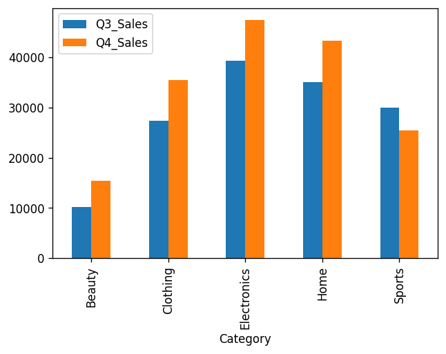
That’s not a bad-looking plot. Especially considering we wrote just one line of code to generate it!
We can also customize this plot using the formatting parameters. Let’s add the figure title and the axis labels. And make product categories easier to read:
category_sales.plot.bar(
    xlabel='Product Category',
    ylabel='Sales (in dollars)',
    title='FIG 1: Sales by Category',
    rot=45 # rotate xticks by 45 degrees
)
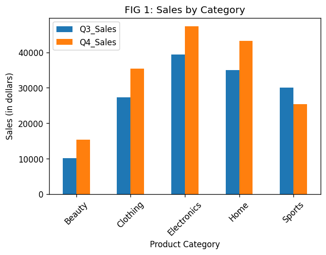
The total sales went up from Q3 to Q4 for all the categories except Sports. Let’s look at the data from another angle for a different perspective.
Plot Pie Chart
The above bar plot compares the Q3 and Q4 sales for each category. We could also look at how much each category contributed within each quarter.
Pie charts would be the perfect visualization tool for that. Let’s draw them by invoking the pie() method on the category_sales DataFrame.
We’ll use two key parameters4 to get the desired result:
subplots: draw separate pie charts for Q3 and Q4 sales.autopct: print percentage of sales contributed by each category.
axes = category_sales.plot.pie(
    figsize=(12,6),
    subplots=True, # show Q3 and Q4 side by side
    autopct='%1.2f%%', # show percent of each slice
    legend=None,
    title='FIG 2: Sales by Category - Q3 vs. Q4'
)
# Add x and y axis label for both charts
axes[0].set_xlabel('Q3 Sales')
axes[0].set_ylabel('')
axes[1].set_xlabel('Q4 Sales')
axes[1].set_ylabel('')
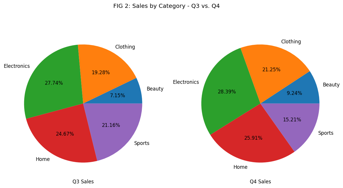
The share of the Sports category went down from 21.16% in Q3 to 15.21% in Q4. That’s a significant drop! Store management should look into it.
Create A New Column
The DataFrame sales_df has the Q3 and Q4 sales data. We might also want to know the percent change in sales from Q3 to Q4.
We can calculate that using the below formula:
Let’s apply this formula on the sales_df5 and store the results in a new column Pct_Change:
# Find the change in sales from Q3 to Q4
diff = sales_df['Q4_Sales'] - sales_df['Q3_Sales']
# Calculate percentage change and add a new column for it
sales_df['Pct_Change'] = (diff*100) / sales_df['Q3_Sales']
And print the first five rows to confirm that sales_df now contains the new column:
sales_df.head()| Category | Q3_Sales | Q4_Sales | Pct_Change | |
|---|---|---|---|---|
| Department | ||||
| Haircare | Beauty | 1529 | 2254 | 47.42 |
| Kitchen | Home | 4638 | 5792 | 24.88 |
| TVs | Electronics | 9270 | 11215 | 20.98 |
| Football | Sports | 8915 | 5694 | -36.13 |
| Men | Clothing | 4497 | 5906 | 31.33 |
Let’s filter the rows where the percent change is negative and sort them:
# Find entries where percent change is negative
# and sorted by low to high
sales_df.query('Pct_Change < 0').sort_values('Pct_Change')| Category | Q3_Sales | Q4_Sales | Pct_Change | |
|---|---|---|---|---|
| Department | ||||
| Tennis | Sports | 4605 | 2270 | -50.71 |
| Football | Sports | 8915 | 5694 | -36.13 |
| Baseball | Sports | 8290 | 6531 | -21.22 |
| Refurbished | Electronics | 1334 | 1297 | -2.77 |
These are the worst-performing departments. Three of them are from the Sports category.
That doesn’t surprise us. In the last section, we already saw that the total Sports sales shrunk significantly compared to other categories.
Save DataFrame to CSV File
We’ve made quite a few changes to sales_df since we loaded it from the original CSV file. We can save the updated DataFrame to a new file using the to_csv() method:
# Persist the sales_df DataFrame to a CSV file
# in your current local directory
sales_df.to_csv('retail_sales_profits_v2.csv')
By default, this method will persist the index as well. You can set the parameter index to False if you want to exclude the index.
Summary
Pandas is an essential tool for performing data analysis in Python. This tutorial has provided you with the foundational knowledge of Pandas and its most important features and methods.
Here’s a quick recap of what you learned today:
- read_csv(): Load CSV dataset as a DataFrame.
- head() & tail(): Take a peek at the DataFrame.
- set_index(): Set a column as the index.
- info(): Print useful information about the DataFrame.
- describe(): Get summary statistics for the numerical data.
- unique() & value_counts(): Summarize categorical columns.
- rename() & set_axis(): Update column labels.
- Select columns using square bracket notation.
- drop(): Remove unnecessary columns.
- Create new columns based on the existing data.
- query(): Filter data using logical expressions.
- sort_values() & sort_index(): Sort data using columns or index.
- Method chaining: Perform multiple operations sequentially.
- groupby(): Group and aggregate data.
- Visualize data using Pandas’ built-in functions (e.g., bar() and pie() )
- to_csv(): Save DataFrame to a CSV file.
You should now have enough practical skills in Pandas to explore simple datasets on your own.
Footnotes
-
Check out Pandas read methods to find the details. ↩
-
Your output may differ from what you see here. That’s because I’ve customized the Pandas’ output using its display options. Here are the options I used:
pd.set_option('display.max_rows', 10)pd.set_option('display.float_format', '{:,.2f}'.format)↩ -
You can learn more about logical expressions and operators here. ↩
-
Check out this article if you want to customize pie charts further. ↩
-
Pandas will perform these operations on all the rows in one shot. Learn more about it here. ↩
Title Image by
Stone Wang