· 8 minute read

How to Read and Write Excel Files Using Pandas
· · 10 minute read
Introduction
We recently covered the basics of Pandas. Today, we’ll learn how to work with Excel spreadsheets using Pandas.
Here’s what this article will cover:
- Read Excel file into a DataFrame.
- Load selected columns and skip blank rows or columns.
- Read multiple worksheets from an Excel file.
- Write a DataFrame to an Excel file.
- Write multiple worksheets to an Excel file.
Datasets
We’ll use below Excel files in today’s tutorial:
- largest_cities.xlsx: contains data on the 200 largest US cities.
- ranked_cities.xlsx: has three worksheets with rankings of US cities.
Please download them from here and copy them to the same directory as your Jupyter Notebook (or Python script).
Install OpenPyXL
Pandas uses the OpenPyXL library to interact with Excel files. You can install it using the below pip command:
# Run this from the command line
pip install openpyxl
Now you can launch your notebook and import Pandas as usual:
# import Pandas library
# It'll import openpyxl automatically when required
import pandas as pd
Read Excel File
We’ll load the Excel file largest_cities.xlsx in this section. Here’s a screenshot of this file:
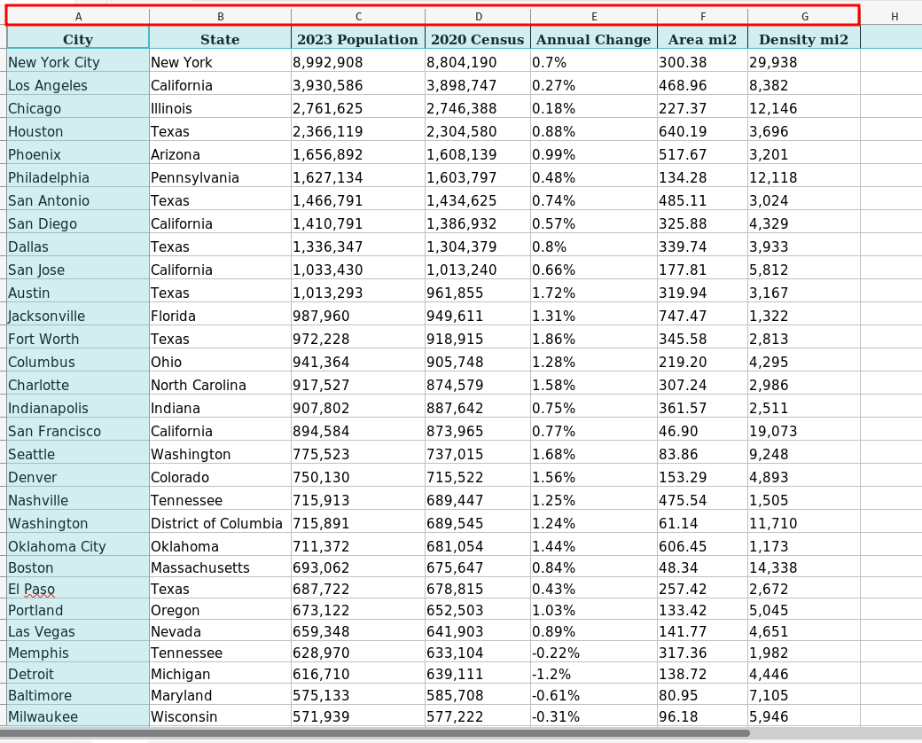
A few important things to notice:
- The first row contains the column headers (City, State, 2023 Population, etc.).
- The first column, City, has the names of the largest US cities. We can use it as an index to identify rows uniquely.
- Excel also assigns alphabetical labels (A, B, C, etc.) to each column (red rectangle). These labels will come in handy, as we’ll see later.
Let’s use Pandas’ method read_excel() to load this file. The method will return a Pandas DataFrame:
# Read the Excel file and print the DataFrame
# Pass the full file path as the input
# we have the file in the same directory as the code
# So, below will work
pd.read_excel('largest_cities.xlsx')| City | State | 2023 Population | 2020 Census | Annual Change |
Area mi2 |
Density mi2 |
|
|---|---|---|---|---|---|---|---|
| 0 | New York City | New York | 8,992,908 | 8,804,190 | 0.7% | 300.38 | 29,938 |
| 1 | Los Angeles | California | 3,930,586 | 3,898,747 | 0.27% | 468.96 | 8,382 |
| 2 | Chicago | Illinois | 2,761,625 | 2,746,388 | 0.18% | 227.37 | 12,146 |
| 3 | Houston | Texas | 2,366,119 | 2,304,580 | 0.88% | 640.19 | 3,696 |
| 4 | Phoenix | Arizona | 1,656,892 | 1,608,139 | 0.99% | 517.67 | 3,201 |
| ... | ... | ... | ... | ... | ... | ... | ... |
| 195 | Torrance | California | 147,556 | 147,067 | 0.11% | 20.52 | 7,190 |
| 196 | Rockford | Illinois | 147,389 | 148,655 | -0.29% | 64.38 | 2,289 |
| 197 | Visalia | California | 146,466 | 141,384 | 1.17% | 37.92 | 3,862 |
| 198 | Fullerton | California | 146,155 | 143,617 | 0.58% | 22.43 | 6,516 |
| 199 | Gainesville | Florida | 146,104 | 141,085 | 1.16% | 63.07 | 2,317 |
200 rows × 7 columns
Pandas used the first row for column labels (in blue). However, it automatically created an index (in red). Let’s print the index to confirm:
# print DataFrame index
largest_cities.index
RangeIndex(start=0, stop=200, step=1)It is a numerical index ranging from 0 to 199. We don’t want that. Instead, we should use the City column (in green) as the index.
.
Set Column as Index
We can set a column (or a list of columns) as the index using the DataFrame method set_index():
# set City as the index
largest_cities = largest_cities.set_index('City')
# print the top 5 rows
largest_cities.head()| State | 2023 Population | 2020 Census | Annual Change |
Area mi2 |
Density mi2 |
|
|---|---|---|---|---|---|---|
| City | ||||||
| New York City | New York | 8,992,908 | 8,804,190 | 0.7% | 300.38 | 29,938 |
| Los Angeles | California | 3,930,586 | 3,898,747 | 0.27% | 468.96 | 8,382 |
| Chicago | Illinois | 2,761,625 | 2,746,388 | 0.18% | 227.37 | 12,146 |
| Houston | Texas | 2,366,119 | 2,304,580 | 0.88% | 640.19 | 3,696 |
| Phoenix | Arizona | 1,656,892 | 1,608,139 | 0.99% | 517.67 | 3,201 |
The DataFrame looks better. The list of cities is set as the index. Let’s print the index again to confirm:
largest_cities.indexIndex(['New York City', 'Los Angeles', 'Chicago', 'Houston', 'Phoenix',
'Philadelphia', 'San Antonio', 'San Diego', 'Dallas', 'San Jose',
...
'Kent', 'Syracuse', 'Thornton', 'Denton', 'Jackson', 'Torrance',
'Rockford', 'Visalia', 'Fullerton', 'Gainesville'],
dtype='object', name='City', length=200)You can now use Pandas loc[] to access specific cities using the index labels:
# Get data for a specific city
# using loc and single square brackets
largest_cities.loc['Anchorage']
State Alaska
2023 Population 291,073
2020 Census 291,247
Annual Change -0.02%
Area mi2 1,706.80
Density mi2 171
Name: Anchorage, dtype: object# Access data for multiple cities
# Notice the use of double square brackets
largest_cities.loc[['Austin', 'Denver', 'Nashville']]| State | 2023 Population | 2020 Census | Annual Change |
Area mi2 |
Density mi2 |
|
|---|---|---|---|---|---|---|
| City | ||||||
| Austin | Texas | 1,013,293 | 961,855 | 1.72% | 319.94 | 3,167 |
| Denver | Colorado | 750,130 | 715,522 | 1.56% | 153.29 | 4,893 |
| Nashville | Tennessee | 715,913 | 689,447 | 1.25% | 475.54 | 1,505 |
Load Selected Columns
Recall that Excel assigns letter labels (A, B, C, etc.) to each column. The read_excel() method allows you to use these labels to load a specific set of columns.
Let’s see some examples.
List of Columns
The parameter usecols takes in a list of comma-separated letter labels to load specific columns.
Suppose you only want to load four specific columns - City, State, 2020 Census, and Density mi2. You can do that by passing their corresponding letter labels to the parameter usecols:
largest_cities = pd.read_excel(
    'largest_cities.xlsx',
    # load specific columns using Excel letter labels
    usecols='A,B,D,G',
    # Use the first loaded column as the index
    index_col=0
)
largest_cities.head()| State | 2020 Census | Density mi2 | |
|---|---|---|---|
| City | |||
| New York City | New York | 8,804,190 | 29,938 |
| Los Angeles | California | 3,898,747 | 8,382 |
| Chicago | Illinois | 2,746,388 | 12,146 |
| Houston | Texas | 2,304,580 | 3,696 |
| Phoenix | Arizona | 1,608,139 | 3,201 |
Consecutive Columns
Suppose you want to load a range of columns (e.g., from A to D). We can use usecols to specify the start and end columns using a colon (:) like below.
largest_cities = pd.read_excel(
    'largest_cities.xlsx',
    # Load columns A to D (both inclusive)
    usecols='A:D',
    # Set the first loaded column as the index
    index_col=0
)
# Print the last five rows from the DataFrame
largest_cities.tail()| State | 2023 Population | 2020 Census | |
|---|---|---|---|
| City | |||
| Torrance | California | 147,556 | 147,067 |
| Rockford | Illinois | 147,389 | 148,655 |
| Visalia | California | 146,466 | 141,384 |
| Fullerton | California | 146,155 | 143,617 |
| Gainesville | Florida | 146,104 | 141,085 |
Mixed Columns
We can also read specific columns and a range of columns together. The below code loads a range (C:E) and two individual columns using usecols:
largest_cities = pd.read_excel(
    'largest_cities.xlsx',
    # load a range and the individual columns
    usecols='A,C:E,G',
    # set the first loaded column as the index
    index_col=0
)
largest_cities.head()| 2023 Population | 2020 Census | Annual Change |
Density mi2 |
|
|---|---|---|---|---|
| City | ||||
| New York City | 8,992,908 | 8,804,190 | 0.7% | 29,938 |
| Los Angeles | 3,930,586 | 3,898,747 | 0.27% | 8,382 |
| Chicago | 2,761,625 | 2,746,388 | 0.18% | 12,146 |
| Houston | 2,366,119 | 2,304,580 | 0.88% | 3,696 |
| Phoenix | 1,656,892 | 1,608,139 | 0.99% | 3,201 |
Read Excel With Blank Rows & Columns
So far, we’ve worked with a perfect Excel file. However, it’s common to get messy excel files with empty rows and columns.
Let’s see an example - largest_cities_blank_rc.xlsx has the same data we saw in the last section, but the first column (A) and the top four rows are blank:
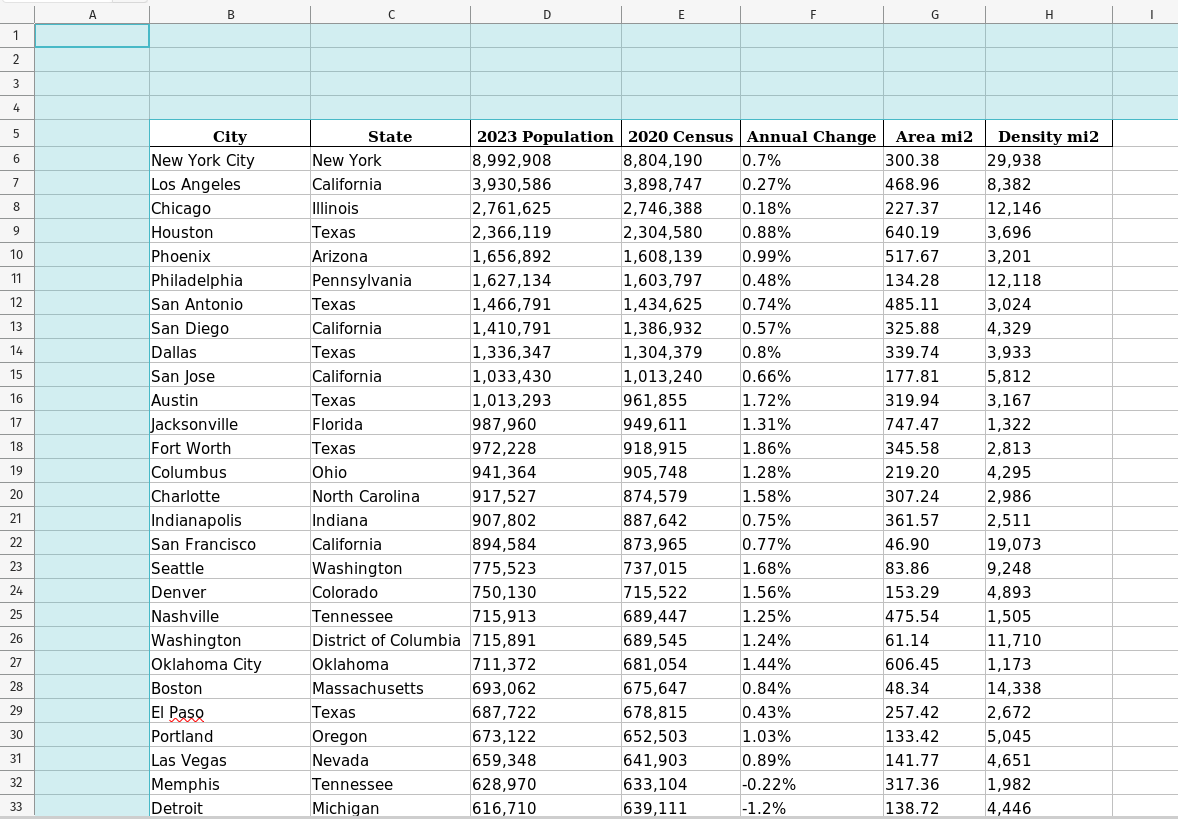
If you load this file using read_excel(), you’ll see a DataFrame with lots of missing values (NaN / Unnamed):
# Load a file with blank rows and columns
pd.read_excel('largest_cities_blank_rc.xlsx')| Unnamed: 0 | Unnamed: 1 | Unnamed: 2 | Unnamed: 3 | Unnamed: 4 | Unnamed: 5 | Unnamed: 6 | Unnamed: 7 | |
|---|---|---|---|---|---|---|---|---|
| 0 | NaN | NaN | NaN | NaN | NaN | NaN | NaN | NaN |
| 1 | NaN | NaN | NaN | NaN | NaN | NaN | NaN | NaN |
| 2 | NaN | NaN | NaN | NaN | NaN | NaN | NaN | NaN |
| 3 | NaN | City | State | 2023 Population | 2020 Census | Annual Change | Area mi2 | Density mi2 |
| 4 | NaN | New York City | New York | 8,992,908 | 8,804,190 | 0.7% | 300.38 | 29,938 |
| ... | ... | ... | ... | ... | ... | ... | ... | ... |
| 199 | NaN | Torrance | California | 147,556 | 147,067 | 0.11% | 20.52 | 7,190 |
| 200 | NaN | Rockford | Illinois | 147,389 | 148,655 | -0.29% | 64.38 | 2,289 |
| 201 | NaN | Visalia | California | 146,466 | 141,384 | 1.17% | 37.92 | 3,862 |
| 202 | NaN | Fullerton | California | 146,155 | 143,617 | 0.58% | 22.43 | 6,516 |
| 203 | NaN | Gainesville | Florida | 146,104 | 141,085 | 1.16% | 63.07 | 2,317 |
204 rows × 8 columns
You can skip these empty rows and columns using the below parameters:
- usecols: We already covered this parameter in the last section. Since columns B to H contain the data, we’ll set it to ‘B:H’.
- skiprows: The number of lines to skip at the start of the file. We know the file begins with four blank rows, so let’s set it to 4.
pd.read_excel(
    'largest_cities_blank_rc.xlsx',
    # Skip the first four rows
    skiprows=4,
    # Load columns B to H (thus skip A)
    usecols='B:H',
    # Use the first loaded column as the index
    index_col=0
)| State | 2023 Population | 2020 Census | Annual Change |
Area mi2 |
Density mi2 |
|
|---|---|---|---|---|---|---|
| City | ||||||
| New York City | New York | 8,992,908 | 8,804,190 | 0.7% | 300.38 | 29,938 |
| Los Angeles | California | 3,930,586 | 3,898,747 | 0.27% | 468.96 | 8,382 |
| Chicago | Illinois | 2,761,625 | 2,746,388 | 0.18% | 227.37 | 12,146 |
| Houston | Texas | 2,366,119 | 2,304,580 | 0.88% | 640.19 | 3,696 |
| Phoenix | Arizona | 1,656,892 | 1,608,139 | 0.99% | 517.67 | 3,201 |
| ... | ... | ... | ... | ... | ... | ... |
| Torrance | California | 147,556 | 147,067 | 0.11% | 20.52 | 7,190 |
| Rockford | Illinois | 147,389 | 148,655 | -0.29% | 64.38 | 2,289 |
| Visalia | California | 146,466 | 141,384 | 1.17% | 37.92 | 3,862 |
| Fullerton | California | 146,155 | 143,617 | 0.58% | 22.43 | 6,516 |
| Gainesville | Florida | 146,104 | 141,085 | 1.16% | 63.07 | 2,317 |
200 rows × 7 columns
The DataFrame looks good now. It doesn’t have any empty rows or columns, and it uses City as the index.
Read Excel With Multiple Sheets
Excel files can have multiple worksheets, each containing a different data set.
Pandas works great with such files. It helps you to:
- Get the names of all the sheets in a file.
- Load a specific sheet or a selected set of sheets.
- Load all sheets.
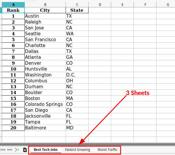
Let’s see these operations in action. We’ll use the excel file ranked_cities.xlsx, which contains three sheets:
Get Sheet Names
How can you get the names of all the sheets in an Excel file?
Easy! Load the file using the ExcelFile class. Then get the value of the sheet_names attribute:
# Get the names of all the sheets in an Excel spreadsheet
pd.ExcelFile('ranked_cities.xlsx').sheet_names
['Best Tech Jobs', 'Fastest Growing', 'Worst Traffic']Load Specific Sheet
By default, the read_excel() method loads the first sheet from the Excel file:
# by default, read_excel() loads the first sheet
ranked_cities = pd.read_excel(
    # load the first sheet - 'Best Tech Jobs'
    'ranked_cities.xlsx',
    # Use the loaded sheet's first column
    # as the index
    index_col=0
)
ranked_cities.head()| City | State | |
|---|---|---|
| Rank | ||
| 1 | Austin | TX |
| 2 | Raleigh | NC |
| 3 | San Jose | CA |
| 4 | Seattle | WA |
| 5 | San Francisco | CA |
You can load a specific sheet by using the parameter sheet_name:
ranked_cities = pd.read_excel(
    'ranked_cities.xlsx',
    # load a specific sheet
    sheet_name='Fastest Growing',
    # Set the first column as the index
    index_col=0
)
ranked_cities.head() # Fastest Growing| City | State | |
|---|---|---|
| Rank | ||
| 1 | Seattle | WA |
| 2 | Austin | TX |
| 3 | Forth Worth | TX |
| 4 | Miami | FL |
| 5 | Denver | CO |
Load selected sheets
The parameter sheet_name is quite versatile. It also accepts a list of sheet names (or their integer positions).
For example, if you want to load the first and third sheets, you can set sheet_name to ['Best Tech Jobs', 'Worst Traffic'], or [0, 2]. You’ll get back a dictionary containing data from both sheets.
ranked_cities =  pd.read_excel(
    'ranked_cities.xlsx',
    # sheet_name - Sheets to load
    # Accepts integer index as well
    # so sheet_name=[0, 2] will load the same sheets
    sheet_name=['Best Tech Jobs', 'Worst Traffic'],
    # Set the first column as the index
    # for all loaded sheets
    index_col=0
)

# Check return type - it must be a dictionary
type(ranked_cities)dictLet’s print the dictionary keys. It’ll be the same sheet names (or integer positions) that you passed in the above read_excel() call.
ranked_cities.keys()dict_keys(['Best Tech Jobs', 'Worst Traffic'])The dictionary values will be the DataFrame objects for each sheet. Let’s retrieve them:
# Get DataFrame objects from the dictionary
tech_df = ranked_cities['Best Tech Jobs']
traffic_df = ranked_cities['Worst Traffic']
And print the top 5 entries from both DataFrames:
# Top 5 cities for tech jobs
tech_df.head()| City | State | |
|---|---|---|
| Rank | ||
| 1 | Austin | TX |
| 2 | Raleigh | NC |
| 3 | San Jose | CA |
| 4 | Seattle | WA |
| 5 | San Francisco | CA |
# Top 5 cities with the worst traffic
traffic_df.head()| City | State | Hours | |
|---|---|---|---|
| Rank | |||
| 1 | Boston | MA | 164 |
| 2 | Washington | D.C. | 155 |
| 3 | Chicago | IL | 138 |
| 4 | New York City | NY | 133 |
| 5 | Los Angeles | CA | 128 |
Los Angeles in the fifth position? That’s shocking 😲. It’s impossible to imagine a city with worse traffic than LA!
Load All Sheets
You can read all the sheets at once by setting sheet_name to None:
ranked_cities =  pd.read_excel(
    'ranked_cities.xlsx',
    # Load all the sheets
    sheet_name=None,
    # Set the first column as
    # the index for all sheets
    index_col=0
)
The returned dictionary will now have all three sheets:
ranked_cities.keys()dict_keys(['Best Tech Jobs', 'Fastest Growing', 'Worst Traffic'])Let’s print the DataFrame containing the fastest growing cities:
ranked_cities['Fastest Growing'].head()| City | State | |
|---|---|---|
| Rank | ||
| 1 | Seattle | WA |
| 2 | Austin | TX |
| 3 | Forth Worth | TX |
| 4 | Miami | FL |
| 5 | Denver | CO |
Write DataFrame to Excel File
Pandas makes it easy to save DataFrames as Excel files. Let’s see it in action.
Suppose you’ve compiled a list of your favorite restaurants in Seattle. And you prepare a DataFrame with their cuisine type and customer ratings:
seattle_restaurants = [
    ['Bakery Nouveau', 'French', 4.6],
    ['Pizzeria Credo', 'Italian', 4.6],
    ['Chan Seattle', 'Korean', 4.4],
    ['Tilikum Place Cafe', 'European', 4.6],
    ['Ba Bar Capitol Hill', 'Vietnamese', 4.5]
]

seattle_restaurants_df = pd.DataFrame(
    data=seattle_restaurants,
    columns=['Restaurant', 'Cuisine', 'Rating']
)

# Print DataFrame contents
seattle_restaurants_df| Restaurant | Cuisine | Rating | |
|---|---|---|---|
| 0 | Bakery Nouveau | French | 4.6 |
| 1 | Pizzeria Credo | Italian | 4.6 |
| 2 | Chan Seattle | Korean | 4.4 |
| 3 | Tilikum Place Cafe | European | 4.6 |
| 4 | Ba Bar Capitol Hill | Vietnamese | 4.5 |
You can write this DataFrame to an Excel file using the method to_excel().
It’ll persist the index as well. We don’t want to save the numeric index. So we’ll set the parameter index to False:
seattle_restaurants_df.to_excel(
    'seattle_restaurants.xlsx',
    # Don't save the auto-generated numeric index
    index=False
)
You should now see the file seattle_restaurants.xlsx in the same directory where you’re running this notebook.
Write Multiple sheets
Suppose you also compile a list of restaurants in New York City:
nyc_restaurants = [
    ['Piccola Cucina Estiatorio', 'Italian', 4.6],
    ['Boucherie West Village', 'French', 4.6],
    ['Mei Jin Ramen', 'Japanese', 4.5],
    ['Spice Symphony', 'Indian', 4.4],
    ['Bua Thai Ramen & Robata Grill', 'Thai', 4.5]
]

nyc_restaurants_df = pd.DataFrame(
    data=nyc_restaurants,
    columns=['Restaurant', 'Cuisine', 'Rating']
)

nyc_restaurants_df| Restaurant | Cuisine | Rating | |
|---|---|---|---|
| 0 | Piccola Cucina Estiatorio | Italian | 4.6 |
| 1 | Boucherie West Village | French | 4.6 |
| 2 | Mei Jin Ramen | Japanese | 4.5 |
| 3 | Spice Symphony | Indian | 4.4 |
| 4 | Bua Thai Ramen & Robata Grill | Thai | 4.5 |
Now you have two DataFrames with lists of your favorite restaurants in two cities - seattle_restaurants_df and nyc_restaurants_df.
You would like to create an Excel file with two sheets - it should have one sheet for each DataFrame. You can do that by using Pandas’ class ExcelWriter and DataFrame method to_excel():
# Create an ExcelWriter instance
# and use it as a context manager
with pd.ExcelWriter('cities_restaurants.xlsx') as writer:
    # Write Seattle restaurants to a sheet named 'Seattle'
    seattle_restaurants_df.to_excel(
        writer,
        sheet_name='Seattle',
        index=False
    )
    # Write NYC restaurants to a sheet named 'New York City'
    nyc_restaurants_df.to_excel(
        writer,
        sheet_name='New York City',
        index=False
    )
You’ll now see a new Excel file, cities_restaurants.xlsx, in your current directory. And it’ll have two sheets - Seattle and New York City.
Add Sheet to Existing File
Let’s say you gather a list of restaurants in New Orleans and create a DataFrame for them:
# New Orleans - Favorite restaurants
nola_restaurants = [
    ['Olde Nola Cookery', 'Cajun & Creole', 4.4],
    ['Atchafalaya', 'Contemporary', 4.7],
    ['Southern Candymakers', 'Dessert', 4.7],
    ['Maïs Arepas', 'Colombian', 4.5],
    ['Katie\'s Restaurant & Bar', 'Cajun & Creole', 4.6]
]

nola_restaurants_df = pd.DataFrame(
    data=nola_restaurants,
    columns=['Restaurant', 'Cuisine', 'Rating'])

nola_restaurants_df| Restaurant | Cuisine | Rating | |
|---|---|---|---|
| 0 | Olde Nola Cookery | Cajun & Creole | 4.4 |
| 1 | Atchafalaya | Contemporary | 4.7 |
| 2 | Southern Candymakers | Dessert | 4.7 |
| 3 | Maïs Arepas | Colombian | 4.5 |
| 4 | Katie's Restaurant & Bar | Cajun & Creole | 4.6 |
And you want to save this DataFrame as a new sheet in the file we created in the last section - cities_restaurants.xlsx.
To do that, you’ll need to use the class ExcelWriter in append mode (parameter mode='a'):
# Add a new sheet to the existing file
# Create an instance of ExcelWriter in append mode
with pd.ExcelWriter('cities_restaurants.xlsx', mode='a') as writer:
    # Append new sheet
    nola_restaurants_df.to_excel(
        writer,
        sheet_name='New Orleans',
        index=False
    )
Let’s confirm that the Excel file has the new sheet by printing the sheet names:
# Print the names of all the sheets in the Excel file
pd.ExcelFile('cities_restaurants.xlsx').sheet_names
['Seattle', 'New York City', 'New Orleans']As expected, the file now contains the new sheet - New Orleans.
Summary
This article showed you how to interact with Excel files using Python and Pandas. Here’s a quick recap of what we learned today:
- Read Excel files using read_excel().
- Load selected columns using the parameter
usecols. - Skip blank columns and rows with the parameters
usecolsandskiprows. - Read selected sheets using the parameter
sheet_name.
- Load selected columns using the parameter
- Write DataFrame to Excel file using to_excel().
- Create an Excel file with multiple sheets with the class ExcelWriter.
Title Image by
Scott Webb