· 6 minute read

Precision, Recall, and F1 Score: A Practical Guide Using Scikit-Learn
· · 7 minute read
Introduction
In the last post, we learned why Accuracy could be a misleading metric for classification problems with imbalanced classes. And how Precision, Recall, and F1 Score can come to our rescue.
It’s time to put all that theory into practice using Python, Scikit-Learn, and Seaborn.
First, let me introduce the dataset we’ll be working with today.
Credit Card Default Dataset
We’ll use the Default dataset from ISLR. The dataset1 contains credit card debt information for 10,000 consumers and has the following columns:
- default: indicates whether the consumer defaulted on the debt (0 - didn’t default, 1 - defaulted).
- student: indicates whether the consumer is a student (0 - No, 1 - Yes).
- balance: consumer’s credit card balance.
- income: consumer’s annual income.
We aim is to build a classification model to predict whether consumers will default on their credit card debts.
Let’s dive in!
First Classification Model
Load the dataset
First, we load the dataset using pandas:
import pandas as pd

dataset = pd.read_csv('Default.csv')
dataset.info()
<class 'pandas.core.frame.DataFrame'>
RangeIndex: 10000 entries, 0 to 9999
Data columns (total 4 columns):
# Column Non-Null Count Dtype
--- ------ -------------- -----
0 default 10000 non-null int64
1 student 10000 non-null int64
2 balance 10000 non-null float64
3 income 10000 non-null float64
dtypes: float64(2), int64(2)
memory usage: 312.6 KBAs expected, the dataset contains observations for 10K consumers. Moreover, every column has 10K non-null values. So we don’t have any missing data.
Imbalanced Classes
Next, let’s find out how many consumers have defaulted on their loans.
We can use Pandas’ function value_counts() to get the counts of each outcome in default, the output column:
dataset['default'].value_counts()0 9667
1 333
Name: default, dtype: int64Only 333 out of 10K, or 3.33% of consumers have defaulted on their loans. We are dealing with a dataset with imbalanced classes. This will become important, as we’ll see later.
Train Test Split
Let’s store input columns (student, balance, and income) as variable X, and output column (default) as y:
# X contains all input columns
# Use pandas drop() to get all columns except 'default'
X = dataset.drop(columns='default')

# y has the output column
y = dataset['default']
We must ensure that we’ll test our model on data it has never seen during training. So let’s set aside a portion of the available data for testing.
We’ll use Scikit-Learn’s train_test_split which will return training set (X_train, y_train) and test set (X_test, y_test):
from sklearn.model_selection import train_test_split

# keep 30% of data for testing using the argument 'test_size'
# Order of the output variables is important
X_train, X_test, y_train, y_test = train_test_split(
    X, y, test_size=0.3)
Build the Model
Let’s train the model using Scikit-Learn’s LogisticRegression. Make sure that we use the training data (X_train and y_train) in this phase:
from sklearn.linear_model import LogisticRegression

# liblinear solver works well with unscaled data
model = LogisticRegression(solver='liblinear')
# fit the model on the training data
model.fit(X_train, y_train)
Evaluate the Model
Now that the model is fully trained, let’s measure its performance. We’ll use the model to predict the output (default) for all test inputs, X_test:
# predict y for the test inputs
y_test_predictions = model.predict(X_test)
Plot Confusion Matrix
Next, let’s generate a Confusion Matrix by comparing the actual test output (y_test) with the model’s predictions (y_test_predictions):
# import all the metrics we'll use later on
from sklearn.metrics import (
    confusion_matrix,
    accuracy_score,
    precision_score,
    recall_score,
    f1_score
)

# Generate confusion matrix for the predictions
conf_matrix = confusion_matrix(y_test, y_test_predictions)
conf_matrix
array([[2907, 2],
[ 91, 0]])The above output can be hard to interpret - it’s just a bunch of numbers in a two-dimensional array.
We can visualize the Confusion Matrix instead using Seaborn heatmap():
import matplotlib.pyplot as plt
import seaborn as sns

plt.figure(figsize=(8,8))
sns.set(font_scale = 1.5)

ax = sns.heatmap(
    conf_matrix, # confusion matrix 2D array
    annot=True, # show numbers in the cells
    fmt='d', # show numbers as integers
    cbar=False, # don't show the color bar
    cmap='flag', # customize color map
    vmax=175 # to get better color contrast
)

ax.set_xlabel("Predicted", labelpad=20)
ax.set_ylabel("Actual", labelpad=20)
plt.show()
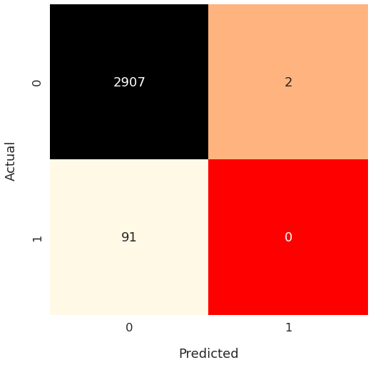
Notice the bottom left square (containing the number 91).
The test set contained 91 cases where consumers defaulted on their loans (actual value = 1). Our model couldn’t predict any of them correctly (predicted value = 0).
That’s a terrible performance! Let’s see if Accuracy reflects this reality.
accuracy = accuracy_score(y_test, y_test_predictions)
print(f"Accuracy = {accuracy}")
Accuracy = 0.969No, it doesn’t. A model which gets all the positive cases wrong isn’t supposed to have an Accuracy of almost 97%.
This paradoxical phenomenon where a model has high Accuracy but performs poorly is known as the Accuracy Paradox.
That’s why you cannot trust Accuracy to measure the performance of a classification model. That’s especially true when you have imbalanced classes.
We’ll turn to the metrics that can help us identify bad models in such situations.
Precision, Recall, and F1 Score
Let’s calculate Precision, Recall, and F1 Score using Scikit-Learn’s built-in functions - precision_score(), recall_score() and f1_score().
precision = precision_score(y_test, y_test_predictions)
recall = recall_score(y_test, y_test_predictions)
f1score = f1_score(y_test, y_test_predictions)

print(f"Precision = {precision}")
print(f"Recall = {recall}")
print(f"F1 Score = {f1score}")
Precision = 0.0
Recall = 0.0
F1 Score = 0.0All of them are 0. That’s not surprising. We know our model is flawed, as it failed to predict any of the positive cases.
A Better Model
The model we built performed terribly because the input dataset had imbalanced classes.
How can we mitigate the harmful effect of imbalanced classes? One way is to assign a higher weight to the observations that occur infrequently.
LogisticsRegression can do that if you use the parameter class_weight and set its value to balanced.
Let’s build another model using this option. Then get new predictions for the test input data X_test.
model = LogisticRegression(
    solver='liblinear',
    class_weight='balanced' # handle imbalanced classes
)
# fit the model on the training data
model.fit(X_train, y_train)
# and then predict y for the test inputs
y_test_predictions = model.predict(X_test)
Next, plot the Confusion Matrix for the test predictions:
conf_matrix = confusion_matrix(y_test, y_test_predictions)

plt.figure(figsize=(8,8))
sns.set(font_scale = 1.5)

ax = sns.heatmap(
    conf_matrix, annot=True, fmt='d',
    cbar=False, cmap='tab10', vmax=500
)

ax.set_xlabel("Predicted", labelpad=20)
ax.set_ylabel("Actual", labelpad=20)
plt.show()
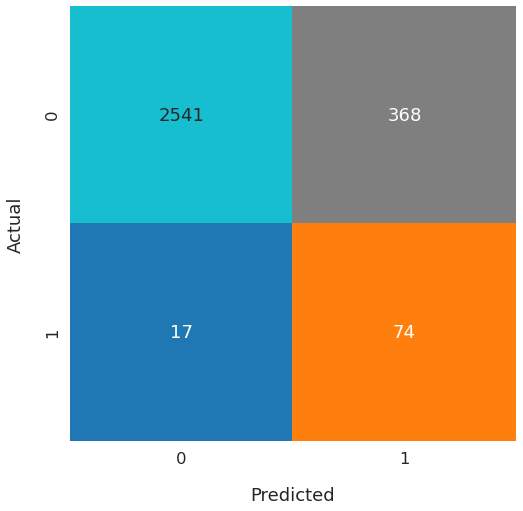
The new model correctly predicted 74 of the 91 positive cases. That’s quite an improvement!
Let’s calculate the performance metrics for the new model:
accuracy = accuracy_score(y_test, y_test_predictions)
precision = precision_score(y_test, y_test_predictions)
recall = recall_score(y_test, y_test_predictions)
f1score = f1_score(y_test, y_test_predictions)

print(f"Accuracy = {accuracy.round(4)}")
print(f"Precision = {precision.round(4)}")
print(f"Recall = {recall.round(4)}")
print(f"F1 Score = {f1score.round(4)}")
Accuracy = 0.8717
Precision = 0.1674
Recall = 0.8132
F1 Score = 0.2777Here's the summary of metrics for both models:
| Metric | First Model | Second Model |
|---|---|---|
| Accuracy | 0.969 | 0.8717 |
| Precision | 0.0 | 0.1674 |
| Recall | 0.0 | 0.8132 |
| F1 Score | 0.0 | 0.2777 |
The second model has much better overall performance. Even though it has slightly lower Accuracy but other scores went up. Especially, Recall has shot up significantly.
There’s room for improvement, though. Precision is still too low. I’ll leave it as an exercise for you to refine the model further.
Summary & Next Steps
This post showed us how to evaluate classification models using Scikit-Learn and Seaborn.
We built a model that suffered from Accuracy Paradox. Then we measured its performance by plotting the Confusion Matrix and calculating Precision, Recall, and F1 Score.
Next, we used Scikit-Learn’s built-in feature to tackle imbalance in the output classes. That helped us train a better-performing model.
Here are a few suggestions if you want to enhance your knowledge of classification metrics:
-
Explore Scikit-Learn’s classification_report().
-
Learn about ROC Curve (Receiver Operating Characteristic Curve) for binary classifiers.
Footnotes
-
We’ll use a slightly modified version of ISLR Default dataset. ↩
Title Image by
anncapictures