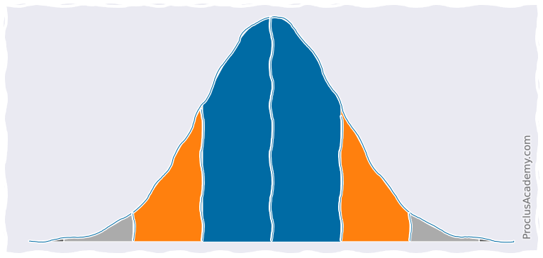
Normal Distribution and the Empirical Rule
Normal Distribution
We covered Data Distributions and Density Curves in recent posts (see here and here).
Now we turn our attention to Normal Distribution - a particular type of distribution used widely in Statistics and Machine Learning.
You can recognize normal distribution by some of its signature features. Let’s explore these features using an example.
The weight of newborn babies is normally distributed. Suppose the mean weight is 7.75 pounds with a standard deviation of 0.85. Then the probability density curve for newborn weights will look like this:
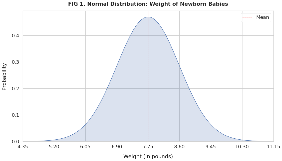
The x-axis has the newborn weights in increasing order. The curve’s height shows the probability (on the y-axis) corresponding to the weight.
Since newborn weight follows a normal distribution, this curve will exhibit some unique properties:
- Mean, median, and mode are the same value and lie at the center (red line).
- Symmetrical: If you split the curve by the mean, the left and the right sides are mirror images of each other.
- Bell Shaped: The curve has a peak at the mean. The probability drops off as you move away from the mean in either direction.
- The curve never touches the x-axis. No matter how far from the center, every value has a probability greater than 0.
- The total area under the curve equals 1. That’s because it represents all possible weight measurements and their probabilities.
Empirical Rule
You’ll notice that the majority of the values in FIG 1 are clustered around the mean.
When a variable follows a normal distribution, almost all of its values occur within three standard deviations from the mean.
To be more precise, 68% of the values fall within one standard deviation, 95% within two, and 99.7% within three standard deviations from the mean.
This is known as the Empirical Rule or 68-95-99.7 Rule.
Let’s apply it to the newborn weights.
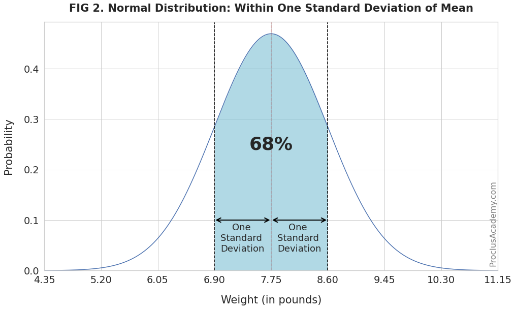
The weight 6.90 pounds is one standard deviation below the mean. And 8.60 pounds is one standard deviation above the mean.
Thus, the empirical rule dictates that 68% of newborn babies will weigh between 6.90 and 8.60 pounds. Below figure shows this information graphically:
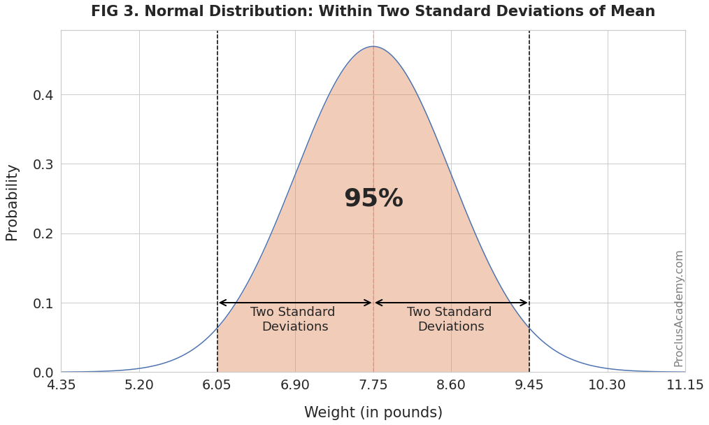
Similarly, 95% of the babies will weigh between 6.05 and 9.45 pounds (two standard deviations from the mean):
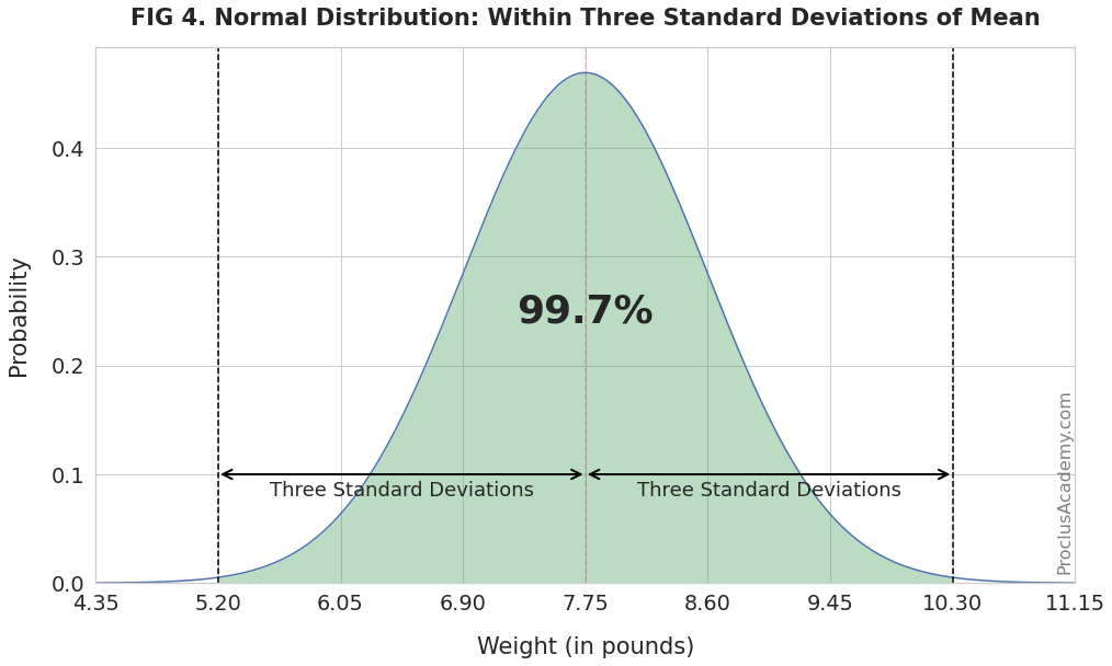
Finally, the weights of almost all (99.7%) newborns will fall between 5.20 and 10.30 pounds (three standard deviations from the mean):
Using the Empirical Rule
Let’s say you want to know:
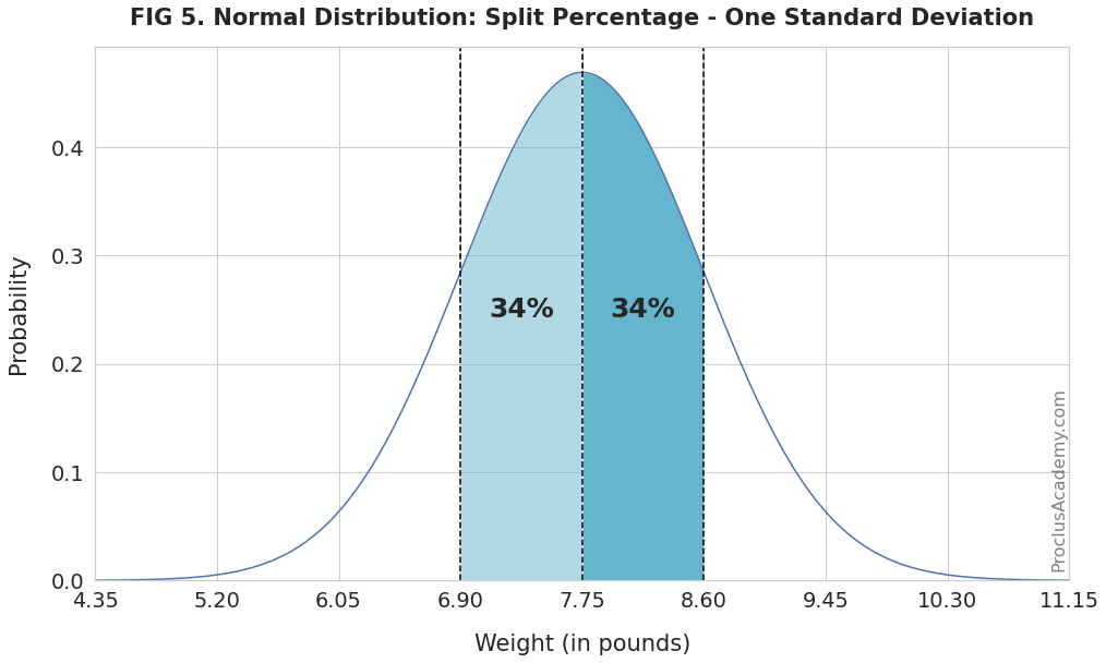
How many newborns weigh between 7.75 pounds (mean) and 8.60 pounds (one standard deviation above the mean)?
We know from FIG 2 that 68% of newborns weigh between one standard deviation below and above the mean. And the weight range in the question above is the right half of the shaded area in FIG 2.
Since the normal distribution is symmetrical about the mean, the left and right half will have equal area and thus equal percentages.
Thus, 34% of the newborns will weigh between 7.75 pounds and 8.60 pounds, as the below figure shows (in the darker blue shade):
You can use the empirical rule and symmetry property to solve a variety of probability problems.
For example, you could calculate probabilities for intervals of one standard deviation as you move away from the mean. The below plot shows the results:
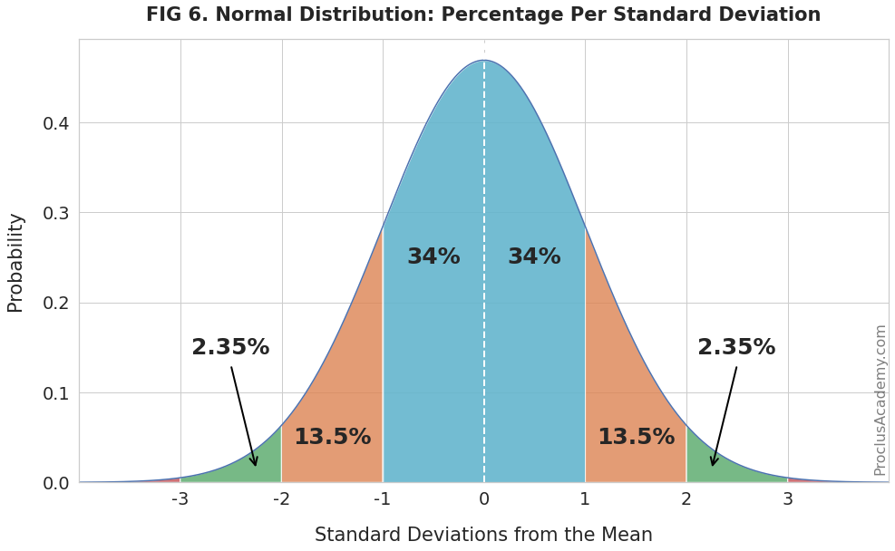
As expected, the probability drops dramatically as the distance from the mean increases.
Summary
This post covered the basics of Normal Distribution. It also introduced Empirical Rule and showed how you could use it.
Check out the next post, where we’ll use Python and SciPy to generate and plot Normal Distributions.