· 10 minute read

Creating Z-Score Tables in Python: A Step-by-Step Guide
· · 9 minute read
Introduction
In a recent article, we covered the concept of z-score and its applications. We also learned about cumulative probability. It is the probability of selecting a random value that is less than or equal to a specific value in a given distribution.
In this article, we’ll cover the z-score table (aka z-table), which is used to find the cumulative probability for a specific z-score in a standard normal distribution1.
I’ll show you how to use a z-score table. Then, we’ll dive into a hands-on session where we’ll create this table in Python using popular data analysis and statistical libraries.
Let’s get started!
Using Z-Score Table
The z-score tables allow us to find the cumulative probabilities for z-scores between to for a normal distribution.
The table arranges the z-scores along the left column and the top row. The left column contains the z-score to one decimal. The top row has the second decimal of the z-score. Each cell in the table shows the cumulative probability for a z-score that’s calculated by adding the row and column headers:
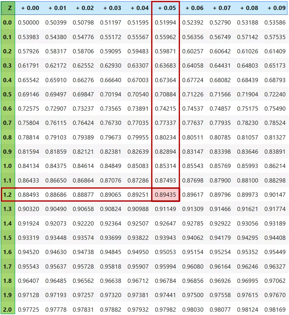
Let me illustrate how to use the z-score table using an example.
Suppose you want to determine the probability that a random value falls below the z-score of . First, we find z-score to one decimal () in the left column. Then, go across that row to the column with the second decimal () at the top. The probability is found in the intersecting cell ().
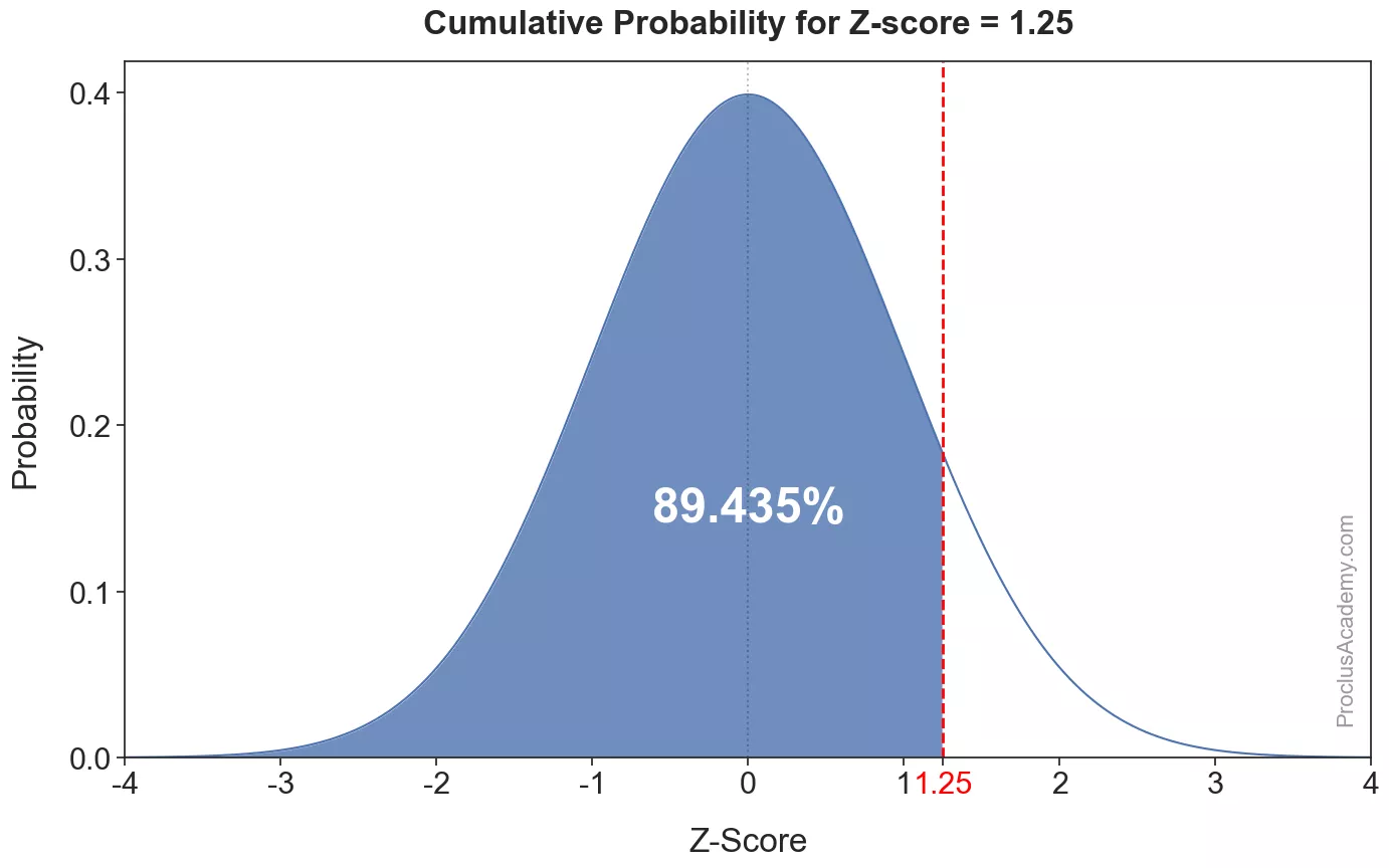
Thus, of values in normal distribution fall below the z-score of . We can depict this using the density curve as well. The below graph shows this cumulative probability as the shaded area to the left of z-score of :
Now that you know how to use the z-score table, let’s create it using Python.
Creating Z-Score Table
The full z-table is usually broken into two tables - one containing probabilities for positive z-scores to and another for the negative z-scores to . The screenshot in the last section showed the positive z-score table.
We’ll first build the table with the positive z-scores. Here are the steps we’ll follow:
- Build a 2-dimensional grid where:
- The left column has the z-score from to in increments of .
- The top row goes from to with a step of .
- Each cell of the grid represents a z-score up to 2 decimals - it is the sum of the corresponding row and column headers (e.g., )
- Find the cumulative probability for the z-score in each cell.
- The resulting grid with the above probabilities is the z-score table.
We’ll implement these steps in Python using the popular libraries for data analysis (NumPy, Pandas) and statistics (SciPy stats).
Let’s start off by importing these libraries:
# Import required libraries
import numpy as np
import scipy.stats as stats
import pandas as pd
Step 1: Create Row and Column Headers
We’ll use NumPy’s arange() function to create the row and column headers. The row headers will contain the z-scores from to , evenly spaced with a step of :
# The row headers (the first column in the table).
# The 2nd parameter (end of interval) is excluded from the output.
# Thus, we'll set it to 4.1 to get values from 0 to 4.
row_headers = np.arange(0, 4.1, 0.1)
row_headers
array([0. , 0.1, 0.2, 0.3, 0.4, 0.5, 0.6, 0.7, 0.8, 0.9, 1. ,
1.1, 1.2, 1.3, 1.4, 1.5, 1.6, 1.7, 1.8, 1.9, 2. ,
2.1, 2.2, 2.3, 2.4, 2.5, 2.6, 2.7, 2.8, 2.9, 3. ,
3.1, 3.2, 3.3, 3.4, 3.5, 3.6, 3.7, 3.8, 3.9, 4. ])And the column headers has the second decimal values :
# The column headers (the first row in the table)
column_headers = np.arange(0.0, 0.10, 0.01)
column_headers
array([0. , 0.01, 0.02, 0.03, 0.04, 0.05, 0.06, 0.07, 0.08, 0.09])Step 2: Create a 2-Dimensional Grid
Next, we want to create a table with all possible combinations of the above two headers. Let’s use NumPy’s meshgrid() for this purpose. It’ll generate a 2D grid with coordinate pairs for each combination of row and column headers.
# Generate a 2D grid of column and row headers.
# It'll return two 2D arrays containing pairs for
# for each combination of row and column headers.
X1, X2 = np.meshgrid(column_headers, row_headers)
When we add X1 and X2, we’ll get the grid of z-scores values of 2 decimal places. Let’s look at the first 5 rows:
z_score_grid = X1 + X2
z_score_grid[:5]
array([[0. , 0.01, 0.02, 0.03, 0.04, 0.05, 0.06, 0.07, 0.08, 0.09],
[0.1 , 0.11, 0.12, 0.13, 0.14, 0.15, 0.16, 0.17, 0.18, 0.19],
[0.2 , 0.21, 0.22, 0.23, 0.24, 0.25, 0.26, 0.27, 0.28, 0.29],
[0.3 , 0.31, 0.32, 0.33, 0.34, 0.35, 0.36, 0.37, 0.38, 0.39],
[0.4 , 0.41, 0.42, 0.43, 0.44, 0.45, 0.46, 0.47, 0.48, 0.49]])And the last 5 rows:
z_score_grid[-5:]array([[3.6 , 3.61, 3.62, 3.63, 3.64, 3.65, 3.66, 3.67, 3.68, 3.69],
[3.7 , 3.71, 3.72, 3.73, 3.74, 3.75, 3.76, 3.77, 3.78, 3.79],
[3.8 , 3.81, 3.82, 3.83, 3.84, 3.85, 3.86, 3.87, 3.88, 3.89],
[3.9 , 3.91, 3.92, 3.93, 3.94, 3.95, 3.96, 3.97, 3.98, 3.99],
[4. , 4.01, 4.02, 4.03, 4.04, 4.05, 4.06, 4.07, 4.08, 4.09]])We’ve got the grid of evenly spaced z-scores going from to . Lets move to the next step.
Step 3: Calculate Cumulative Probability
The norm.cdf() function from SciPy stats returns the cumulative probability for a given z-score in a normal distribution. Let’s use it for the z-score of :
# Find the cumulative
stats.norm.cdf(1.25)0.8943502263331446About % of values fall below the z-score of 1.25. This is the same result we saw earlier.
Applying norm.cdf() to z_score_grid will return a 2D array containing the cumulative probability for all z-scores:
# Get cumulative probability for all the z-scores.
z_score_cdf_grid = stats.norm.cdf(z_score_grid)
# Print the first five rows
z_score_cdf_grid[:5]
array([[0.5 , 0.50398936, 0.50797831, 0.51196647, 0.51595344,
0.51993881, 0.52392218, 0.52790317, 0.53188137, 0.53585639],
[0.53982784, 0.54379531, 0.54775843, 0.55171679, 0.55567 ,
0.55961769, 0.56355946, 0.56749493, 0.57142372, 0.57534543],
[0.57925971, 0.58316616, 0.58706442, 0.59095412, 0.59483487,
0.59870633, 0.60256811, 0.60641987, 0.61026125, 0.61409188],
[0.61791142, 0.62171952, 0.62551583, 0.62930002, 0.63307174,
0.63683065, 0.64057643, 0.64430875, 0.64802729, 0.65173173],
[0.65542174, 0.65909703, 0.66275727, 0.66640218, 0.67003145,
0.67364478, 0.67724189, 0.68082249, 0.6843863 , 0.68793305]])Next, let’s convert the above 2D array into a pandas DataFrame and set the row and column headers. That’ll make it easy to look up the probability for a given z-score:
positive_z_score_table = pd.DataFrame(
    # Pass the z-score CDF 2D array
    z_score_cdf_grid,
    # Set the single decimal z-scores as the index
    index=row_headers,
    # Set array with 2nd decimal as the columns header
    columns=column_headers
)
# Print the first 5 rows
positive_z_score_table.head()| 0.00 | 0.01 | 0.02 | 0.03 | 0.04 | 0.05 | 0.06 | 0.07 | 0.08 | 0.09 | |
|---|---|---|---|---|---|---|---|---|---|---|
| 0.0 | 0.500000 | 0.503989 | 0.507978 | 0.511966 | 0.515953 | 0.519939 | 0.523922 | 0.527903 | 0.531881 | 0.535856 |
| 0.1 | 0.539828 | 0.543795 | 0.547758 | 0.551717 | 0.555670 | 0.559618 | 0.563559 | 0.567495 | 0.571424 | 0.575345 |
| 0.2 | 0.579260 | 0.583166 | 0.587064 | 0.590954 | 0.594835 | 0.598706 | 0.602568 | 0.606420 | 0.610261 | 0.614092 |
| 0.3 | 0.617911 | 0.621720 | 0.625516 | 0.629300 | 0.633072 | 0.636831 | 0.640576 | 0.644309 | 0.648027 | 0.651732 |
| 0.4 | 0.655422 | 0.659097 | 0.662757 | 0.666402 | 0.670031 | 0.673645 | 0.677242 | 0.680822 | 0.684386 | 0.687933 |
Let’s make a few more improvements. We’ll add a plus sign in front of the column header values. That’ll indicate that we need to add the z-score from the row header to the nd decimal value found in the column header. We’ll also round all the probabilities to 5 decimals:
# Format the column headers - add leading + sign
formatted_cols = [f"+ {col:.2f}" for col in column_headers]
positive_z_score_table.columns = formatted_cols

# round all probability values to 5 decimals
positive_z_score_table.round(5)| + 0.00 | + 0.01 | + 0.02 | + 0.03 | + 0.04 | + 0.05 | + 0.06 | + 0.07 | + 0.08 | + 0.09 | |
|---|---|---|---|---|---|---|---|---|---|---|
| 0.0 | 0.50000 | 0.50399 | 0.50798 | 0.51197 | 0.51595 | 0.51994 | 0.52392 | 0.52790 | 0.53188 | 0.53586 |
| 0.1 | 0.53983 | 0.54380 | 0.54776 | 0.55172 | 0.55567 | 0.55962 | 0.56356 | 0.56749 | 0.57142 | 0.57535 |
| 0.2 | 0.57926 | 0.58317 | 0.58706 | 0.59095 | 0.59483 | 0.59871 | 0.60257 | 0.60642 | 0.61026 | 0.61409 |
| 0.3 | 0.61791 | 0.62172 | 0.62552 | 0.62930 | 0.63307 | 0.63683 | 0.64058 | 0.64431 | 0.64803 | 0.65173 |
| 0.4 | 0.65542 | 0.65910 | 0.66276 | 0.66640 | 0.67003 | 0.67364 | 0.67724 | 0.68082 | 0.68439 | 0.68793 |
| 0.5 | 0.69146 | 0.69497 | 0.69847 | 0.70194 | 0.70540 | 0.70884 | 0.71226 | 0.71566 | 0.71904 | 0.72240 |
| 0.6 | 0.72575 | 0.72907 | 0.73237 | 0.73565 | 0.73891 | 0.74215 | 0.74537 | 0.74857 | 0.75175 | 0.75490 |
| 0.7 | 0.75804 | 0.76115 | 0.76424 | 0.76730 | 0.77035 | 0.77337 | 0.77637 | 0.77935 | 0.78230 | 0.78524 |
| 0.8 | 0.78814 | 0.79103 | 0.79389 | 0.79673 | 0.79955 | 0.80234 | 0.80511 | 0.80785 | 0.81057 | 0.81327 |
| 0.9 | 0.81594 | 0.81859 | 0.82121 | 0.82381 | 0.82639 | 0.82894 | 0.83147 | 0.83398 | 0.83646 | 0.83891 |
| 1.0 | 0.84134 | 0.84375 | 0.84614 | 0.84849 | 0.85083 | 0.85314 | 0.85543 | 0.85769 | 0.85993 | 0.86214 |
| 1.1 | 0.86433 | 0.86650 | 0.86864 | 0.87076 | 0.87286 | 0.87493 | 0.87698 | 0.87900 | 0.88100 | 0.88298 |
| 1.2 | 0.88493 | 0.88686 | 0.88877 | 0.89065 | 0.89251 | 0.89435 | 0.89617 | 0.89796 | 0.89973 | 0.90147 |
| 1.3 | 0.90320 | 0.90490 | 0.90658 | 0.90824 | 0.90988 | 0.91149 | 0.91309 | 0.91466 | 0.91621 | 0.91774 |
| 1.4 | 0.91924 | 0.92073 | 0.92220 | 0.92364 | 0.92507 | 0.92647 | 0.92785 | 0.92922 | 0.93056 | 0.93189 |
| 1.5 | 0.93319 | 0.93448 | 0.93574 | 0.93699 | 0.93822 | 0.93943 | 0.94062 | 0.94179 | 0.94295 | 0.94408 |
| 1.6 | 0.94520 | 0.94630 | 0.94738 | 0.94845 | 0.94950 | 0.95053 | 0.95154 | 0.95254 | 0.95352 | 0.95449 |
| 1.7 | 0.95543 | 0.95637 | 0.95728 | 0.95818 | 0.95907 | 0.95994 | 0.96080 | 0.96164 | 0.96246 | 0.96327 |
| 1.8 | 0.96407 | 0.96485 | 0.96562 | 0.96638 | 0.96712 | 0.96784 | 0.96856 | 0.96926 | 0.96995 | 0.97062 |
| 1.9 | 0.97128 | 0.97193 | 0.97257 | 0.97320 | 0.97381 | 0.97441 | 0.97500 | 0.97558 | 0.97615 | 0.97670 |
| 2.0 | 0.97725 | 0.97778 | 0.97831 | 0.97882 | 0.97932 | 0.97982 | 0.98030 | 0.98077 | 0.98124 | 0.98169 |
| 2.1 | 0.98214 | 0.98257 | 0.98300 | 0.98341 | 0.98382 | 0.98422 | 0.98461 | 0.98500 | 0.98537 | 0.98574 |
| 2.2 | 0.98610 | 0.98645 | 0.98679 | 0.98713 | 0.98745 | 0.98778 | 0.98809 | 0.98840 | 0.98870 | 0.98899 |
| 2.3 | 0.98928 | 0.98956 | 0.98983 | 0.99010 | 0.99036 | 0.99061 | 0.99086 | 0.99111 | 0.99134 | 0.99158 |
| 2.4 | 0.99180 | 0.99202 | 0.99224 | 0.99245 | 0.99266 | 0.99286 | 0.99305 | 0.99324 | 0.99343 | 0.99361 |
| 2.5 | 0.99379 | 0.99396 | 0.99413 | 0.99430 | 0.99446 | 0.99461 | 0.99477 | 0.99492 | 0.99506 | 0.99520 |
| 2.6 | 0.99534 | 0.99547 | 0.99560 | 0.99573 | 0.99585 | 0.99598 | 0.99609 | 0.99621 | 0.99632 | 0.99643 |
| 2.7 | 0.99653 | 0.99664 | 0.99674 | 0.99683 | 0.99693 | 0.99702 | 0.99711 | 0.99720 | 0.99728 | 0.99736 |
| 2.8 | 0.99744 | 0.99752 | 0.99760 | 0.99767 | 0.99774 | 0.99781 | 0.99788 | 0.99795 | 0.99801 | 0.99807 |
| 2.9 | 0.99813 | 0.99819 | 0.99825 | 0.99831 | 0.99836 | 0.99841 | 0.99846 | 0.99851 | 0.99856 | 0.99861 |
| 3.0 | 0.99865 | 0.99869 | 0.99874 | 0.99878 | 0.99882 | 0.99886 | 0.99889 | 0.99893 | 0.99896 | 0.99900 |
| 3.1 | 0.99903 | 0.99906 | 0.99910 | 0.99913 | 0.99916 | 0.99918 | 0.99921 | 0.99924 | 0.99926 | 0.99929 |
| 3.2 | 0.99931 | 0.99934 | 0.99936 | 0.99938 | 0.99940 | 0.99942 | 0.99944 | 0.99946 | 0.99948 | 0.99950 |
| 3.3 | 0.99952 | 0.99953 | 0.99955 | 0.99957 | 0.99958 | 0.99960 | 0.99961 | 0.99962 | 0.99964 | 0.99965 |
| 3.4 | 0.99966 | 0.99968 | 0.99969 | 0.99970 | 0.99971 | 0.99972 | 0.99973 | 0.99974 | 0.99975 | 0.99976 |
| 3.5 | 0.99977 | 0.99978 | 0.99978 | 0.99979 | 0.99980 | 0.99981 | 0.99981 | 0.99982 | 0.99983 | 0.99983 |
| 3.6 | 0.99984 | 0.99985 | 0.99985 | 0.99986 | 0.99986 | 0.99987 | 0.99987 | 0.99988 | 0.99988 | 0.99989 |
| 3.7 | 0.99989 | 0.99990 | 0.99990 | 0.99990 | 0.99991 | 0.99991 | 0.99992 | 0.99992 | 0.99992 | 0.99992 |
| 3.8 | 0.99993 | 0.99993 | 0.99993 | 0.99994 | 0.99994 | 0.99994 | 0.99994 | 0.99995 | 0.99995 | 0.99995 |
| 3.9 | 0.99995 | 0.99995 | 0.99996 | 0.99996 | 0.99996 | 0.99996 | 0.99996 | 0.99996 | 0.99997 | 0.99997 |
| 4.0 | 0.99997 | 0.99997 | 0.99997 | 0.99997 | 0.99997 | 0.99997 | 0.99998 | 0.99998 | 0.99998 | 0.99998 |
This is the z-score table you’ll find in most statistics textbooks and online resources.
Negative Z-Score Table
So far, we have constructed the table for positive z-scores ( to ). Let’s build a similar table for the negative z-scores ( to ). We’ll follow the steps from the last section, but with a few modifications.
The row and column headers will contain negative values. First, prepare row headers with the negative z-scores from to , going up evenly by :
# Row headers from -4 to 0, with a step of 0.1
# The 2nd parameter (end of interval) is excluded from the output.
# Thus, we'll set it to 0.01 to get values from -4 to 0.
row_headers = np.arange(-4, 0.01, 0.1).round(2)
row_headers
array([-4. , -3.9, -3.8, -3.7, -3.6, -3.5, -3.4, -3.3, -3.2, -3.1,
-3. , -2.9, -2.8, -2.7, -2.6, -2.5, -2.4, -2.3, -2.2, -2.1,
-2. , -1.9, -1.8, -1.7, -1.6, -1.5, -1.4, -1.3, -1.2, -1.1,
-1. , -0.9, -0.8, -0.7, -0.6, -0.5, -0.4, -0.3, -0.2, -0.1,
0. ])And prepare the column headers going from to , with a step of :
# From 0.0 to -0.09 with a step of -0.01
column_headers = np.arange(0.0, -0.10, -0.01)
column_headers
array([ 0. , -0.01, -0.02, -0.03, -0.04, -0.05, -0.06, -0.07, -0.08,
-0.09])Next, use NumPy’s meshgrid() to create a 2D grid with all the possible combinations of above row and column headers:
# Generate coordinate pairs for each combination of
# row and column headers
X1, X2 = np.meshgrid(column_headers, row_headers)
Finally, calculate the cumulative probability of each cell in the grid using SciPy norm.cdf(). And convert the output into a pandas DataFrame with appropriate headers:
# Add the coordinates in each cell and
# get cumulative probability for the sum
z_score_cdf_grid = stats.norm.cdf(X1 + X2)

# Prepare pandas dataframe
negative_z_score_table = pd.DataFrame(
    z_score_cdf_grid,
    index=row_headers,
    columns=column_headers
)

# Round the probabilities to 5 decimals
negative_z_score_table.round(5)| 0.00 | -0.01 | -0.02 | -0.03 | -0.04 | -0.05 | -0.06 | -0.07 | -0.08 | -0.09 | |
|---|---|---|---|---|---|---|---|---|---|---|
| -4.0 | 0.00003 | 0.00003 | 0.00003 | 0.00003 | 0.00003 | 0.00003 | 0.00002 | 0.00002 | 0.00002 | 0.00002 |
| -3.9 | 0.00005 | 0.00005 | 0.00004 | 0.00004 | 0.00004 | 0.00004 | 0.00004 | 0.00004 | 0.00003 | 0.00003 |
| -3.8 | 0.00007 | 0.00007 | 0.00007 | 0.00006 | 0.00006 | 0.00006 | 0.00006 | 0.00005 | 0.00005 | 0.00005 |
| -3.7 | 0.00011 | 0.00010 | 0.00010 | 0.00010 | 0.00009 | 0.00009 | 0.00008 | 0.00008 | 0.00008 | 0.00008 |
| -3.6 | 0.00016 | 0.00015 | 0.00015 | 0.00014 | 0.00014 | 0.00013 | 0.00013 | 0.00012 | 0.00012 | 0.00011 |
| -3.5 | 0.00023 | 0.00022 | 0.00022 | 0.00021 | 0.00020 | 0.00019 | 0.00019 | 0.00018 | 0.00017 | 0.00017 |
| -3.4 | 0.00034 | 0.00032 | 0.00031 | 0.00030 | 0.00029 | 0.00028 | 0.00027 | 0.00026 | 0.00025 | 0.00024 |
| -3.3 | 0.00048 | 0.00047 | 0.00045 | 0.00043 | 0.00042 | 0.00040 | 0.00039 | 0.00038 | 0.00036 | 0.00035 |
| -3.2 | 0.00069 | 0.00066 | 0.00064 | 0.00062 | 0.00060 | 0.00058 | 0.00056 | 0.00054 | 0.00052 | 0.00050 |
| -3.1 | 0.00097 | 0.00094 | 0.00090 | 0.00087 | 0.00084 | 0.00082 | 0.00079 | 0.00076 | 0.00074 | 0.00071 |
| -3.0 | 0.00135 | 0.00131 | 0.00126 | 0.00122 | 0.00118 | 0.00114 | 0.00111 | 0.00107 | 0.00104 | 0.00100 |
| -2.9 | 0.00187 | 0.00181 | 0.00175 | 0.00169 | 0.00164 | 0.00159 | 0.00154 | 0.00149 | 0.00144 | 0.00139 |
| -2.8 | 0.00256 | 0.00248 | 0.00240 | 0.00233 | 0.00226 | 0.00219 | 0.00212 | 0.00205 | 0.00199 | 0.00193 |
| -2.7 | 0.00347 | 0.00336 | 0.00326 | 0.00317 | 0.00307 | 0.00298 | 0.00289 | 0.00280 | 0.00272 | 0.00264 |
| -2.6 | 0.00466 | 0.00453 | 0.00440 | 0.00427 | 0.00415 | 0.00402 | 0.00391 | 0.00379 | 0.00368 | 0.00357 |
| -2.5 | 0.00621 | 0.00604 | 0.00587 | 0.00570 | 0.00554 | 0.00539 | 0.00523 | 0.00508 | 0.00494 | 0.00480 |
| -2.4 | 0.00820 | 0.00798 | 0.00776 | 0.00755 | 0.00734 | 0.00714 | 0.00695 | 0.00676 | 0.00657 | 0.00639 |
| -2.3 | 0.01072 | 0.01044 | 0.01017 | 0.00990 | 0.00964 | 0.00939 | 0.00914 | 0.00889 | 0.00866 | 0.00842 |
| -2.2 | 0.01390 | 0.01355 | 0.01321 | 0.01287 | 0.01255 | 0.01222 | 0.01191 | 0.01160 | 0.01130 | 0.01101 |
| -2.1 | 0.01786 | 0.01743 | 0.01700 | 0.01659 | 0.01618 | 0.01578 | 0.01539 | 0.01500 | 0.01463 | 0.01426 |
| -2.0 | 0.02275 | 0.02222 | 0.02169 | 0.02118 | 0.02068 | 0.02018 | 0.01970 | 0.01923 | 0.01876 | 0.01831 |
| -1.9 | 0.02872 | 0.02807 | 0.02743 | 0.02680 | 0.02619 | 0.02559 | 0.02500 | 0.02442 | 0.02385 | 0.02330 |
| -1.8 | 0.03593 | 0.03515 | 0.03438 | 0.03362 | 0.03288 | 0.03216 | 0.03144 | 0.03074 | 0.03005 | 0.02938 |
| -1.7 | 0.04457 | 0.04363 | 0.04272 | 0.04182 | 0.04093 | 0.04006 | 0.03920 | 0.03836 | 0.03754 | 0.03673 |
| -1.6 | 0.05480 | 0.05370 | 0.05262 | 0.05155 | 0.05050 | 0.04947 | 0.04846 | 0.04746 | 0.04648 | 0.04551 |
| -1.5 | 0.06681 | 0.06552 | 0.06426 | 0.06301 | 0.06178 | 0.06057 | 0.05938 | 0.05821 | 0.05705 | 0.05592 |
| -1.4 | 0.08076 | 0.07927 | 0.07780 | 0.07636 | 0.07493 | 0.07353 | 0.07215 | 0.07078 | 0.06944 | 0.06811 |
| -1.3 | 0.09680 | 0.09510 | 0.09342 | 0.09176 | 0.09012 | 0.08851 | 0.08691 | 0.08534 | 0.08379 | 0.08226 |
| -1.2 | 0.11507 | 0.11314 | 0.11123 | 0.10935 | 0.10749 | 0.10565 | 0.10383 | 0.10204 | 0.10027 | 0.09853 |
| -1.1 | 0.13567 | 0.13350 | 0.13136 | 0.12924 | 0.12714 | 0.12507 | 0.12302 | 0.12100 | 0.11900 | 0.11702 |
| -1.0 | 0.15866 | 0.15625 | 0.15386 | 0.15151 | 0.14917 | 0.14686 | 0.14457 | 0.14231 | 0.14007 | 0.13786 |
| -0.9 | 0.18406 | 0.18141 | 0.17879 | 0.17619 | 0.17361 | 0.17106 | 0.16853 | 0.16602 | 0.16354 | 0.16109 |
| -0.8 | 0.21186 | 0.20897 | 0.20611 | 0.20327 | 0.20045 | 0.19766 | 0.19489 | 0.19215 | 0.18943 | 0.18673 |
| -0.7 | 0.24196 | 0.23885 | 0.23576 | 0.23270 | 0.22965 | 0.22663 | 0.22363 | 0.22065 | 0.21770 | 0.21476 |
| -0.6 | 0.27425 | 0.27093 | 0.26763 | 0.26435 | 0.26109 | 0.25785 | 0.25463 | 0.25143 | 0.24825 | 0.24510 |
| -0.5 | 0.30854 | 0.30503 | 0.30153 | 0.29806 | 0.29460 | 0.29116 | 0.28774 | 0.28434 | 0.28096 | 0.27760 |
| -0.4 | 0.34458 | 0.34090 | 0.33724 | 0.33360 | 0.32997 | 0.32636 | 0.32276 | 0.31918 | 0.31561 | 0.31207 |
| -0.3 | 0.38209 | 0.37828 | 0.37448 | 0.37070 | 0.36693 | 0.36317 | 0.35942 | 0.35569 | 0.35197 | 0.34827 |
| -0.2 | 0.42074 | 0.41683 | 0.41294 | 0.40905 | 0.40517 | 0.40129 | 0.39743 | 0.39358 | 0.38974 | 0.38591 |
| -0.1 | 0.46017 | 0.45620 | 0.45224 | 0.44828 | 0.44433 | 0.44038 | 0.43644 | 0.43251 | 0.42858 | 0.42465 |
| 0.0 | 0.50000 | 0.49601 | 0.49202 | 0.48803 | 0.48405 | 0.48006 | 0.47608 | 0.47210 | 0.46812 | 0.46414 |
There you have it. We’ve created the negative z-score table as well!
We now have two z-score tables - one with positive z-scores ( to ) and another with negative z-scores ( to ). Together, these tables allow us to find the cumulative probability for any z-score from to .
Summary
In this article, you learned about the z-score tables and how to use them to find cumulative probability for any given z-score. Then we created the z-score tables using Python, NumPy, SciPy, and pandas.
While it’s true that you can easily find these tables online, the process of creating them from scratch deepens your understanding of z-score and normal distribution, and allows you to customize them for any purpose. This invaluable combination of conceptual knowledge and practical skills provides you with a strong foundation for advanced data and statistical analysis.
Footnotes
-
A standard normal distribution is a normal distribution with a mean of and a standard deviation of . ↩
Title Image by
Schwoaze